【pytorch入門】オーディオI / Oおよびtorchaudioによる前処理(> <;)

表題のとおり、以下の参考ページのコードを動かしてみました。
特に参考になるかというと難しいけど、一応動いたのでまとめておきます。
※歯切れ悪いですが、最後に落ちが、。。。

【参考】
①AUDIO I/O AND PRE-PROCESSING WITH TORCHAUDIO
②TORCHAUDIO.TRANSFORMS
③SOURCE CODE FOR TORCHAUDIO.TRANSFORMS

この項の売りは以下の通りです。
「機械学習の問題を解決するための多大な努力は、データの準備に費やされます。 torchaudioはPyTorchのGPUサポートを活用し、データの読み込みを簡単で読みやすくするための多くのツールを提供します。
このチュートリアルでは、単純なデータセットからデータをロードして前処理する方法を説明します。詳細については、オーディオI / Oおよびtorchaudioによる前処理をご覧ください。
このチュートリアルでは、視覚化を容易にするためにmatplotlibパッケージがインストールされていることを確認してください。」

やったこと

・準備
・Opening a file
・Transformations
・Functional
・Migrating to torchaudio from Kaldi
・Available Datasets

・準備

# Uncomment the following line to run in Google Colab
# !pip install torchaudio
import torch
import torchaudio
import requests
import matplotlib.pyplot as plt

初めて動かすときは以下をインストールする必要があります。

pip install torchaudio

また、ファイルの読込をしようとすると、エラーを吐いて読み込みません。
cannot import torch audio ' No audio backend is available.'
なので、上記のリンクの通り、
Windows fileに対しては、

pip install PySoundFile

Linuxでは、

pip install sox

・Opening a file

「torchaudioは、wavおよびmp3形式のサウンドファイルのロードもサポートしています。波形（waveform）を生のオーディオ信号と呼びます。」
以下のコードは、r = requests.get(url)でurlに存在するwavファイルをrに読み込んで、その後'steam-train-whistle-daniel_simon-converted-from-mp3.wav'として、ローカルに格納します。
※中身は汽笛のようです
そして、再度waveform, sample_rate = torchaudio.load(filename)でデータをwaveformとsample_rateに読み込みます。このwaveformが生のオーディオ信号と呼ぶということです。
※つまり、ローカルにwavファイルを置けば、このコードで読み込めます

url = "https://pytorch.org/tutorials/_static/img/steam-train-whistle-daniel_simon-converted-from-mp3.wav"
r = requests.get(url)

with open('steam-train-whistle-daniel_simon-converted-from-mp3.wav', 'wb') as f:
    f.write(r.content)

filename = "steam-train-whistle-daniel_simon-converted-from-mp3.wav"
waveform, sample_rate = torchaudio.load(filename)

print("Shape of waveform: {}".format(waveform.size()))
print("Sample rate of waveform: {}".format(sample_rate))

plt.figure()
plt.plot(waveform.t().numpy())

そして、plt.plot(waveform.t().numpy())で描画しています。
結果は以下のとおり描画されます。

当初は、なんで重なって二つ出るんだろと思いましたが、標準出力を見ると
Shape of waveform: torch.Size([2, 276858])
Sample rate of waveform: 44100
となっており、torch.Sizeが2になっており、276858のデータが二つあることが分かります。つまり、2chのデータ(stereo data)です。
ということで、描画もわけてやると以下のとおり描画されます。

・Transformations

「torchaudioは、現在も増え続けていますが、以下のリストのような変換をサポートしています。」

関数	機能
Resample:	波形を別のサンプルレートでリサンプリングします。
Spectrogram:	波形からスペクトログラムを作成します。
GriffinLim:	Griffin-Lim変換を使用して、線形スケールのマグニチュードスペクトログラムから波形を計算します。
ComputeDeltas:	テンソル（通常はスペクトログラム）のデルタ係数を計算します
ComplexNorm:	複素テンソルのノルムを計算します。
MelScale:	変換行列を使用して、通常のSTFTをメル周波数STFTに変換されます。
AmplitudeToDB:	これにより、スペクトログラムをパワー/振幅スケールからデシベルスケールに変換します。
MFCC:	波形からメル周波数ケプストラム係数を作成します。
MelSpectrogram:	PyTorchのSTFT関数を使用して、波形からMELスペクトログラムを作成します。
MuLawEncoding:	mu-law圧伸に基づいて波形をエンコードします。
MuLawDecoding:	mu-lawでエンコードされた波形をデコードします。
TimeStretch:	特定のレートでピッチを変更せずに、スペクトログラムを時間内にストレッチします。
FrequencyMasking:	周波数領域のスペクトログラムにマスキングを適用します。
TimeMasking:	時間領域のスペクトログラムにマスキングを適用します。

オリジナルの英文は以下のとおりです。

関数	機能
Resample:	Resample waveform to a different sample rate.
Spectrogram:	Create a spectrogram from a waveform.
GriffinLim:	Compute waveform from a linear scale magnitude spectrogram using the Griffin-Lim transformation.
ComputeDeltas:	Compute delta coefficients of a tensor, usually a spectrogram.
ComplexNorm:	Compute the norm of a complex tensor.
MelScale:	This turns a normal STFT into a Mel-frequency STFT, using a conversion matrix.
AmplitudeToDB:	This turns a spectrogram from the power/amplitude scale to the decibel scale.
MFCC:	Create the Mel-frequency cepstrum coefficients from a waveform.
MelSpectrogram:	Create MEL Spectrograms from a waveform using the STFT function in PyTorch.
MuLawEncoding:	Encode waveform based on mu-law companding.
MuLawDecoding:	Decode mu-law encoded waveform.
TimeStretch:	Stretch a spectrogram in time without modifying pitch for a given rate.
FrequencyMasking:	Apply masking to a spectrogram in the frequency domain.
TimeMasking:	Apply masking to a spectrogram in the time domain.

「各変換はバッチ処理をサポートします。単一の生のオーディオ信号またはスペクトログラム、あるいは同じ形状の多くに対して変換を実行できます。
すべての変換はnn.Modulesまたはjit.ScriptModulesであるため、いつでもニューラルネットワークの一部として使用できます。」

スペクトログラムの対数を対数目盛で見る

specgram = torchaudio.transforms.Spectrogram()(waveform)
print("Shape of spectrogram: {}".format(specgram.size()))
plt.figure()
plt.imshow(specgram.log2()[0,:,:].numpy(), cmap='gray')

※以下はmatplotlibの出力をいじってタイトル出すように変更していますが、コードは煩雑なのでここは載せません。
Shape of spectrogram: torch.Size([2, 201, 1385])
specgram.log2()[0,:,:]で、以下は片方だけ出力しています。

しかし、上記の図がspectorgramっぽく見えますが、信号が汽笛の所為か、特徴無く、判別つきません。そこで、データを以前見た「おはよう、おはよう、おはよう」のwavファイルを読み込んで同じように表示させてみます。
ここで、参考③からtorchaudio.transforms.Spectrogram()の仕様は、以下の通りです。

torchaudio.transforms.Spectrogram(n_fft: int = 400, win_length: Optional[int] = None, hop_length: Optional[int] = None, pad: int = 0, window_fn: Callable[[...], torch.Tensor] = <built-in method hann_window of type object>, power: Optional[float] = 2.0, normalized: bool = False, wkwargs: Optional[dict] = None)

paeameters	type	explaination
n_fft	(int, optional)	– Size of FFT creates n_fft // 2 + 1 bins. (Default: 400)
win_length	(int or None, optional)	– Window size. (Default: n_fft)
hop_length	(int or None, optional)	– Length of hop between STFT windows. (Default: win_length // 2)
pad	(int, optional)	– Two sided padding of signal. (Default: 0)
window_fn	(Callable[.., Tensor], optional)	– A function to create a window tensor that is applied/multiplied to each frame/window. (Default: torch.hann_window)
power	(float or None, optional)	– Exponent for the magnitude spectrogram, (must be > 0) e.g., 1 for energy, 2 for power, etc. If None, then the complex spectrum is returned instead. (Default: 2)
normalized	(bool, optional)	– Whether to normalize by magnitude after stft. (Default: False)
wkwargs	(dict or None, optional)	– Arguments for window function. (Default: None)

上の表から、以下のコードにすると、それなりのspectrogramが出力されました。
※天地も周波数もよくわかりませんが、STFTっぽく見えます。
（以下が入力信号）

（以下がSpectrogramです。この絵は以前「おはよう」のSTFTで得られた絵と同様なものであることが分かります。縦軸のスケールは不明です。）

Shape of spectrogram: torch.Size([1, 513, 431])

filename = "10ohayo0hirakegoma_out.wav" 
waveform, sample_rate = torchaudio.load(filename)
print("Shape of waveform: {}".format(waveform.size()))
print("Sample rate of waveform: {}".format(sample_rate))

sk = "waveform"
fig, (ax1,ax2,ax3) = plt.subplots(3,1,figsize=(1.6180 * 4, 4*2))
lns1=ax1.plot(waveform.t().numpy(),"red",label = "waveform[0]")
lns2=ax2.plot(waveform.t().numpy(),"red",label = "waveform[0]")
lns3=ax3.plot(waveform.t().numpy(),"blue",label = "waveform[0]")
ax1.legend(loc=0)
ax2.legend(loc=0)
ax3.legend(loc=0)
ax1.set_title(sk)
ax2.set_xlim(50000,50000+44100*0.0625) #0,44100*0.25
ax3.set_xlim(3*44100,44100*3.0625)
plt.pause(1)
plt.savefig('./fig/fig_{}_double_.png'.format(sk)) 
plt.close()

specgram = torchaudio.transforms.Spectrogram(n_fft=1024)(waveform)
print("Shape of spectrogram: {}".format(specgram.size()))

sk = "specgram"
fig, (ax1,ax2,ax3) = plt.subplots(3,1,figsize=(1.6180 * 4, 4*2))
lns1=ax1.imshow(specgram.log2()[0,:,:].numpy(), cmap='gray') 
lns2=ax2.imshow(specgram.log2()[0,:,:].numpy(), cmap='hsv') 
lns3=ax3.imshow(specgram.log2()[0,:,:].numpy(), cmap='hsv') 

ax2.set_ylim(250,0)
ax3.set_ylim(125,0)
ax1.set_title(sk)

plt.pause(1)
plt.savefig('./fig/fig_{}_double_.png'.format(sk)) 
plt.close()

対数スケールでメルスペクトログラムを見る

次に、メルスペクトログラムを出力します。
MelSpectrogramとは、
内部ではスペクトログラムに対して、メルフィルタバンクと呼ばれるものをかけています
⇒低周波領域を強調するような振幅調整フィルター
　；輝度調整と似たようなフィルター
【参考】
④メルフィルタバンクを理解する
⑤メル尺度@wikipedia
mel尺度は以下のとおり．．．なのでlog2なんですね。

m = 1000\log _2(\frac{f}{1000Hz}+1)

specgram = torchaudio.transforms.MelSpectrogram()(waveform)
print("Shape of spectrogram: {}".format(specgram.size()))
plt.figure()
p = plt.imshow(specgram.log2()[0,:,:].detach().numpy(), cmap='gray')

Shape of spectrogram: torch.Size([2, 128, 1385])
まあ、上記のSpectrogramと似たような絵が出てきますが上記の変換をしているんでしょうね。

そこで、上記のSpectrogramと同じように仕様を確認します。
以下の通りのようです。

torchaudio.transforms.MelSpectrogram(sample_rate: int = 16000, n_fft: int = 400, win_length: Optional[int] = None, hop_length: Optional[int] = None, f_min: float = 0.0, f_max: Optional[float] = None, pad: int = 0, n_mels: int = 128, window_fn: Callable[[...], torch.Tensor] = <built-in method hann_window of type object>, power: Optional[float] = 2.0, normalized: bool = False, wkwargs: Optional[dict] = None)

それぞれのパラメーターの意味も上記のSpectrogramとほぼ同様です。
ただし、Sampling_rateを指定できます。

paeameters	type	explaination
sample_rate	(int, optional)	– Sample rate of audio signal. (Default: 16000)
win_length	(int or None, optional)	– Window size. (Default: n_fft)
hop_length	(int or None, optional)	– Length of hop between STFT windows. (Default: win_length // 2)
n_fft	(int, optional)	– Size of FFT, creates n_fft // 2 + 1 bins. (Default: 400)
f_min	(float, optional)	– Minimum frequency. (Default: 0.)
f_max	(float or None, optional)	– Maximum frequency. (Default: None)
pad	(int, optional)	– Two sided padding of signal. (Default: 0)
n_mels	(int, optional)	– Number of mel filterbanks. (Default: 128)
window_fn	(Callable[.., Tensor], optional)	– A function to create a window tensor that is applied/multiplied to each frame/window. (Default: torch.hann_window)
wkwargs	(Dict[.., ..] or None, optional)	– Arguments for window function. (Default: None)

上の表に基づいて、以下のようなコードで出力します。
※コードの主要な部分を記述すると以下のとおり
sample_rate=44100,n_fft=2048としています。

specgram = torchaudio.transforms.MelSpectrogram(sample_rate=44100,n_fft=2048)(waveform)
print("Shape of MelSpectrogram: {}".format(specgram.size()))

上のspectrogramと同様な波形ですが、縦方向のスケールが小さくなりましたが、分解能は上より良いように見えます。

リサンプリング

一度に1チャンネルずつ波形をリサンプリングできます。
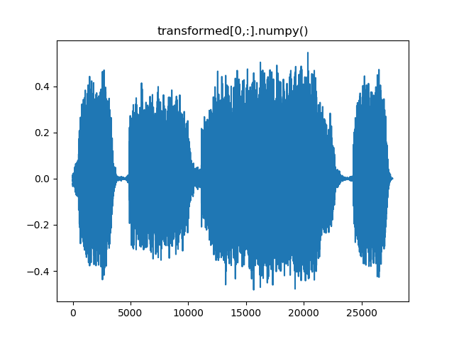
sample_rateを1/10にしています。横軸が元の波形と比較して1/10になっています。

new_sample_rate = sample_rate/10
# Since Resample applies to a single channel, we resample first channel here
channel = 0
transformed = torchaudio.transforms.Resample(sample_rate, new_sample_rate)(waveform[channel,:].view(1,-1))
print("Shape of transformed waveform: {}".format(transformed.size()))
plt.figure()
plt.plot(transformed[0,:].numpy())

Shape of transformed waveform: torch.Size([1, 27686])

μ-Lawアルゴリズム

変換の別の例として、Mu-Lawエンコーディングに基づいて信号をエンコードできます。

※The μ-law algorithm (sometimes written "mu-law", often approximated as "u-law") is a companding algorithm, primarily used in 8-bit PCM digital telecommunication systems in North America and Japan.μ-law algorithm@wikipediaより

ただし、そのためには、信号が-1から1の間である必要があります。テンソルは通常のPyTorchテンソルであるため、標準の演算子を適用できます。」

# Let's check if the tensor is in the interval [-1,1]
print("Min of waveform: {}\nMax of waveform: {}\nMean of waveform: {}".format(waveform.min(), waveform.max(), waveform.mean()))

Min of waveform: -0.572845458984375
Max of waveform: 0.575958251953125
Mean of waveform: 9.293758921558037e-05

「波形はすでに-1と1の間にあるため、正規化する必要はありません。」
以下は、規格化関数です。

def normalize(tensor):
    # Subtract the mean, and scale to the interval [-1,1]
    tensor_minusmean = tensor - tensor.mean()
    return tensor_minusmean/tensor_minusmean.abs().max()
# Let's normalize to the full interval [-1,1]
# waveform = normalize(waveform)

コメントをはずすと、[-1,1]に規格化されます。

「波形のエンコードを適用してみましょう。」

transformed = torchaudio.transforms.MuLawEncoding()(waveform)
print("Shape of transformed waveform: {}".format(transformed.size()))
plt.figure()
plt.plot(transformed[0,:].numpy())

Shape of transformed waveform: torch.Size([2, 276858])

「そして、デコードします。」

reconstructed = torchaudio.transforms.MuLawDecoding()(transformed)
print("Shape of recovered waveform: {}".format(reconstructed.size()))
plt.figure()
plt.plot(reconstructed[0,:].numpy())

Shape of recovered waveform: torch.Size([2, 276858])

「最終的に、元の波形を再構築されたバージョンと比較できます。」

# Compute median relative difference
err = ((waveform-reconstructed).abs() / waveform.abs()).median()
print("Median relative difference between original and MuLaw reconstucted signals: {:.2%}".format(err))

Median relative difference between original and MuLaw reconstucted signals: 1.28%
つまり、圧縮のエンコード・デコードして、誤差が1.28%でした。

Functional

「上記の変換は、計算に低レベルのステートレス関数に依存しています。これらの関数はtorchaudio.functionalで利用できます。完全なリストはこちら(リンク切れ)から入手でき、次のものが含まれます。」
【参考】リンク切れのサイトは以下に変更のようです。
⑥TORCHAUDIO.FUNCTIONAL
残念ながら、Torchaudio.Functionalのページは変更されていて、stftなどは掲載されていません。以下のリンクに存在しているのが分かりました。

functions	内容
istft	: Inverse short time Fourier Transform.
stft	: Short time Fourier Transform.
gain	: Applies amplification or attenuation to the whole waveform.
dither	: Increases the perceived dynamic range of audio stored at a particular bit-depth.
compute_deltas	: Compute delta coefficients of a tensor.
equalizer_biquad	: Design biquad peaking equalizer filter and perform filtering.
lowpass_biquad	: Design biquad lowpass filter and perform filtering.
highpass_biquad	:Design biquad highpass filter and perform filtering.

STFT

ということで、番外編ですが、STFTを試してみました。
まず、仕様は以下のとおりです。

torch.stft(input: torch.Tensor, n_fft: int, hop_length: Optional[int] = None, win_length: Optional[int] = None, window: Optional[torch.Tensor] = None, center: bool = True, pad_mode: str = 'reflect', normalized: bool = False, onesided: Optional[bool] = None, return_complex: Optional[bool] = None) → torch.Tensor

コードは以下のとおりです。
ここで、inputというのがwaveformだろうと思いますが、
Shape of waveform: torch.Size([1, 220160])
であり、inputは、１Dのテンソルか、２Dの(batch, waveform)とのことなので、
waveform.reshape(220160)
と1DにReshapeしました。
描画は以下のように要素1個だけ取り出していますが、シンプルになりました。
lns1=ax1.imshow(specgram.log2().numpy()[:,:,0], cmap='gray')
その結果、暫定的(正しいかどうか不明)ではありますが、以下の図が得られます。

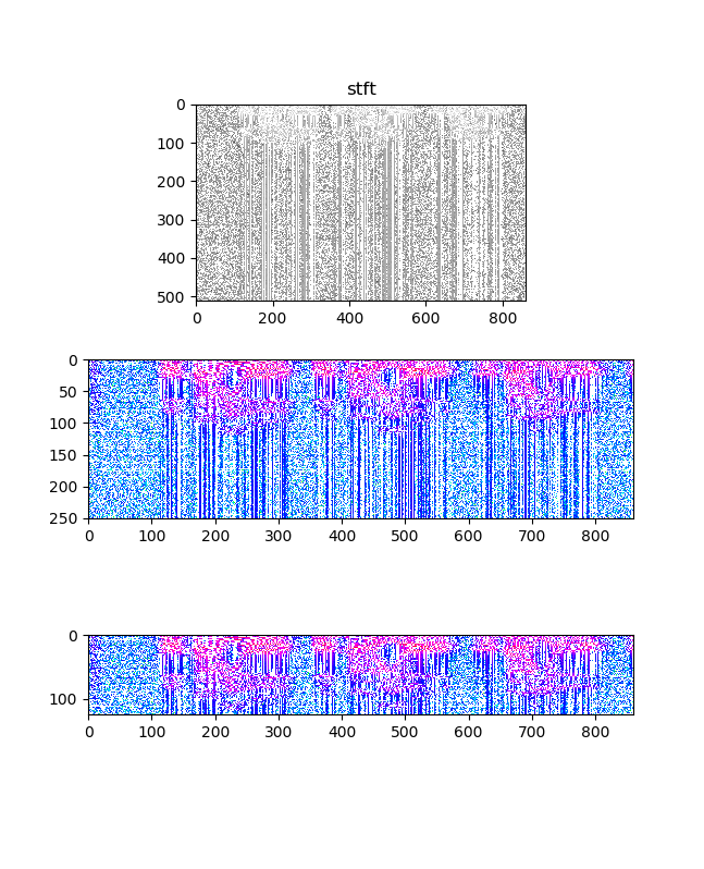
※本来ならソース見て解析するところですが、今回は遠慮しました

sk = "stft"
specgram = torch.stft(input = torch.tensor(waveform.reshape(220160)) ,n_fft=1024) #(waveform)
print("Shape of stftSpectrogram: {}".format(specgram.size()))
fig, (ax1,ax2,ax3) = plt.subplots(3,1,figsize=(1.6180 * 4, 4*2))
lns1=ax1.imshow(specgram.log2().numpy()[:,:,0], cmap='gray')
lns2=ax2.imshow(specgram.log2().numpy()[:,:,0], cmap='hsv')
lns3=ax3.imshow(specgram.log2().numpy()[:,:,0], cmap='hsv')
ax2.set_ylim(250,0)
ax3.set_ylim(125,0)
ax1.set_title(sk)
plt.pause(1)
plt.savefig('./fig/fig_{}_double_.png'.format(sk)) 
plt.close()

※このコードに関しては、以下のコメントあり、これ以上追求しません。
This function changed signature at version 0.4.1. Calling with the previous signature may cause error or return incorrect result.
一方、このstftのソースを読むと以下のコメントが描かれています。

The STFT computes the Fourier transform of short overlapping windows of the input. 
This giving frequency components of the signal as they change over time. 
The interface of this function is modeled after the librosa_ stft function.

    .. _librosa: https://librosa.org/doc/latest/generated/librosa.stft.html

つまり、librosa.stftから設計を拝借したということのようです。
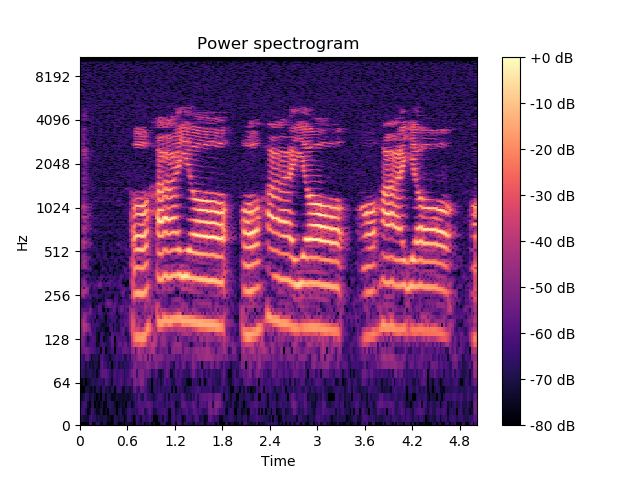
ということで、本家をたたいてみます。こちらは、正しく表示しているようです。

# Feature extraction example
import numpy as np
import librosa
import librosa.display

y, sr = librosa.load('10ohayo0hirakegoma_out.wav')  #trumpet'))

S = np.abs(librosa.stft(y))

S_left = librosa.stft(y, center=False)

D_short = librosa.stft(y, hop_length=64)

import matplotlib.pyplot as plt
fig, ax = plt.subplots()
img = librosa.display.specshow(librosa.amplitude_to_db(S,
                                                       ref=np.max),
                               y_axis='log', x_axis='time', ax=ax)
sk = 'Power spectrogram'
ax.set_title(sk)
fig.colorbar(img, ax=ax, format="%+2.0f dB")
plt.pause(1)
plt.savefig('./fig/fig_{}_librose_.png'.format(sk)) 
plt.close()

こちらは、以下のように縦軸も横軸も信頼できそうな表示を示してくれました。pytorchとは関係ないというか、本来の目的である、GPU使うなどは出来ませんが、一応前処理には使えます。
例）このstft画像を音声認識に利用するための前処理
そして、この図を見られたので上記のグラフが天地でしかもスケールも単に要素数ということが分かりました。

残りの解説がありますが、今回はパスしようと思います。
・mu_law_encoding functional:
・visualize a waveform with the highpass biquad filter.
・Migrating to torchaudio from Kaldi
・create mel frequency cepstral coefficients from a raw audio signal
また、提供されているDatasetsも以下のリンク先の方が新しいような気がします。
・Available Datasets⇒TORCHAUDIO.DATASETS

そして、タイムスタンプみると、以下の通りでした。
© Copyright 2017, PyTorch.
やんぬるかなww

文化になれる（どこに必要な情報があるのかを理解する）のに少し時間がかかるかも．．．

まとめ

・torchaudioを動かしてみた
・gpu計算ができると期待したが、ウワンのマシンではできていない
・タイムスタンプが古いので、出来るだけ新しいページを参照することをお勧めします

因みに以下のページは2017-2018ですね。
© Copyright 2018, Torchaudio Contributors.
TORCHAUDIO
© Copyright 2018, Torchaudio Contributors.
TORCHAUDIO.FUNCTIONAL
© Copyright 2017, PyTorch.
SPEECH COMMAND RECOGNITION WITH TORCHAUDIO