Pythonでインストール出来るというので、遊んでみました。
ほぼ、以下の参考のとおりです。
参考②を真似してpytorch-lightningでグー・チョキ・パーをMLPしてみたのが、特に苦労しました。
つまり、画像とかでなく、普通?の自前データデビュー出来ました。
【参考】
①ML solutions in MediaPipe
②Pythonパッケージ版のMediaPipeが超お手軽 + 簡易なMLPで指ジェスチャー推定
インストールは以下で非常に簡単に入りました。
なお、Raspi4ではversionが未対応とエラーが出て入りませんでした。
pip install mediapipe
やったこと
- 全部動かしてみる??
- handsの詳細
- データ蓄積
- データ分析する(散布図、cos類似度)
- matplotlibでプロットしてみる
- 自前データのdataset, Dataloader
- networkと学習
- predictionしつつ描画
・全部動かしてみる??
上記のページには、15個のML solutionsがあるようですが、そのうちPython対応しているのが、以下の4個のようです。
全部動かしてみました。
大変なように聞こえますが、コードは全て同じような構造なので、分かり易いです。
ということで、動いたコードを以下に並べてみます。
※上記サイトのコードのfor webcam inputの部分のコピーです
Face Mesh
import cv2
import mediapipe as mp
mp_drawing = mp.solutions.drawing_utils
mp_face_mesh = mp.solutions.face_mesh

# For webcam input:
face_mesh = mp_face_mesh.FaceMesh(
    min_detection_confidence=0.5, min_tracking_confidence=0.5)
drawing_spec = mp_drawing.DrawingSpec(thickness=1, circle_radius=1)

cap = cv2.VideoCapture(0)
while cap.isOpened():
    success, image = cap.read()
    if not success:
        print("Ignoring empty camera frame.")
        # If loading a video, use 'break' instead of 'continue'.
        continue
    # Flip the image horizontally for a later selfie-view display, and convert
    # the BGR image to RGB.
    image = cv2.cvtColor(cv2.flip(image, 1), cv2.COLOR_BGR2RGB)
    # To improve performance, optionally mark the image as not writeable to
    # pass by reference.
    image.flags.writeable = False
    results = face_mesh.process(image)
    # Draw the face mesh annotations on the image.
    image.flags.writeable = True
    image = cv2.cvtColor(image, cv2.COLOR_RGB2BGR)
    if results.multi_face_landmarks:
        for face_landmarks in results.multi_face_landmarks:
            mp_drawing.draw_landmarks(
                image=image,
                landmark_list=face_landmarks,
                connections=mp_face_mesh.FACE_CONNECTIONS,
                landmark_drawing_spec=drawing_spec,
                connection_drawing_spec=drawing_spec)
        cv2.imshow('MediaPipe FaceMesh', image)
    if cv2.waitKey(5) & 0xFF == 27:
        break
face_mesh.close()
cap.release()
Hands
import mediapipe as mp
import cv2

mp_drawing = mp.solutions.drawing_utils
mp_hands = mp.solutions.hands
hands = mp_hands.Hands(
    min_detection_confidence=0.7,
    min_tracking_confidence=0.5,
)
cap = cv2.VideoCapture(0)
while cap.isOpened():
    success, image = cap.read()
    if not success:
        print("Ignoring empty camera frame.")
        # If loading a video, use 'break' instead of 'continue'.
        continue
    # Flip the image horizontally for a later selfie-view display, and convert
    # the BGR image to RGB.
    image = cv2.cvtColor(cv2.flip(image, 1), cv2.COLOR_BGR2RGB)
    # To improve performance, optionally mark the image as not writeable to
    # pass by reference.
    image.flags.writeable = False
    results = hands.process(image)
    # Draw the hand annotations on the image.
    image.flags.writeable = True
    image = cv2.cvtColor(image, cv2.COLOR_RGB2BGR)
    image_width, image_height = image.shape[1], image.shape[0]
    if results.multi_hand_landmarks:
        for hand_landmarks in results.multi_hand_landmarks:
            #print('Handedness:', results.multi_handedness)
            mp_drawing.draw_landmarks(image, hand_landmarks, mp_hands.HAND_CONNECTIONS)
            cv2.imshow('MediaPipe Hands', image)
    if cv2.waitKey(5) & 0xFF == 27:
        break
hands.close()
cap.release()
Pose
import mediapipe as mp
import cv2

mp_drawing = mp.solutions.drawing_utils
mp_pose = mp.solutions.pose

pose = mp_pose.Pose(
    min_detection_confidence=0.5, min_tracking_confidence=0.5)
cap = cv2.VideoCapture(0)
while cap.isOpened():
    success, image = cap.read()
    if not success:
        print("Ignoring empty camera frame.")
        # If loading a video, use 'break' instead of 'continue'.
        continue
    # Flip the image horizontally for a later selfie-view display, and convert
    # the BGR image to RGB.
    image = cv2.cvtColor(cv2.flip(image, 1), cv2.COLOR_BGR2RGB)
    # To improve performance, optionally mark the image as not writeable to
    # pass by reference.
    image.flags.writeable = False
    results = pose.process(image)
    # Draw the pose annotation on the image.
    image.flags.writeable = True
    image = cv2.cvtColor(image, cv2.COLOR_RGB2BGR)
    mp_drawing.draw_landmarks(
        image, results.pose_landmarks, mp_pose.POSE_CONNECTIONS)
    cv2.imshow('MediaPipe Pose', image)
    if cv2.waitKey(5) & 0xFF == 27:
        break
hands.close()
cap.release()
Holistic;これが集大成face_mesh+左右Hands+Poseがすべて描画されます
import cv2
import mediapipe as mp

mp_drawing = mp.solutions.drawing_utils
mp_holistic = mp.solutions.holistic
# For webcam input:
holistic = mp_holistic.Holistic(
    min_detection_confidence=0.5, min_tracking_confidence=0.5)
cap = cv2.VideoCapture(0)
while cap.isOpened():
    success, image = cap.read()
    if not success:
        print("Ignoring empty camera frame.")
        # If loading a video, use 'break' instead of 'continue'.
        continue
    # Flip the image horizontally for a later selfie-view display, and convert
    # the BGR image to RGB.
    image = cv2.cvtColor(cv2.flip(image, 1), cv2.COLOR_BGR2RGB)
    # To improve performance, optionally mark the image as not writeable to
    # pass by reference.
    image.flags.writeable = False
    results = holistic.process(image)
    # Draw landmark annotation on the image.
    image.flags.writeable = True
    image = cv2.cvtColor(image, cv2.COLOR_RGB2BGR)
    mp_drawing.draw_landmarks(
        image, results.face_landmarks, mp_holistic.FACE_CONNECTIONS)
    mp_drawing.draw_landmarks(
        image, results.left_hand_landmarks, mp_holistic.HAND_CONNECTIONS)
    mp_drawing.draw_landmarks(
        image, results.right_hand_landmarks, mp_holistic.HAND_CONNECTIONS)
    mp_drawing.draw_landmarks(
        image, results.pose_landmarks, mp_holistic.POSE_CONNECTIONS)
    cv2.imshow('MediaPipe Holistic', image)
    if cv2.waitKey(5) & 0xFF == 27:
        break
holistic.close()
cap.release()
つまり、以下のCamera入力のコードにmediapipeのMLでの分析結果を載せているということです。
上記のコードではミラー像、つまり通常の鏡に映った画像を出力しています。
※以下のコードでは、ミラー像と鏡面像を両方出力するとちょっと変な気持ちがします
Camera base
import cv2

cap = cv2.VideoCapture(0)
while cap.isOpened():
    success, image = cap.read()
    if not success:
        print("Ignoring empty camera frame.")
        # If loading a video, use 'break' instead of 'continue'.
        continue
    #cv2.imshow('Camera', image) #Camera sight
    image = cv2.cvtColor(cv2.flip(image, 1), cv2.COLOR_BGR2RGB)
    image = cv2.cvtColor(image, cv2.COLOR_RGB2BGR)
    cv2.imshow('amera_mirror', image) #Mirror sight
    if cv2.waitKey(5) & 0xFF == 27:
        break
cap.release()
Camera base + face_mesh + hands +pose
import mediapipe as mp
import cv2
import mediapipe as mp
mp_drawing = mp.solutions.drawing_utils

mp_face_mesh = mp.solutions.face_mesh
face_mesh = mp_face_mesh.FaceMesh(
    min_detection_confidence=0.5, min_tracking_confidence=0.5)
drawing_spec = mp_drawing.DrawingSpec(thickness=1, circle_radius=1)

mp_pose = mp.solutions.pose
pose = mp_pose.Pose(
    min_detection_confidence=0.5, min_tracking_confidence=0.5)

mp_hands = mp.solutions.hands
hands = mp_hands.Hands(
    min_detection_confidence=0.7,
    min_tracking_confidence=0.5,
)

image_blank = cv2.imread('blank.jpg') #白紙を台紙にします
sk = 0
cap = cv2.VideoCapture(0)
while cap.isOpened():
    success, image = cap.read()
    image_blank = cv2.imread('blank.jpg')
    if not success:
        print("Ignoring empty camera frame.")
        # If loading a video, use 'break' instead of 'continue'.
        continue
    image = cv2.cvtColor(cv2.flip(image, 1), cv2.COLOR_BGR2RGB)
    cv2.imshow('Camera', image)
    image.flags.writeable = False
    results_face = face_mesh.process(image)
    results_pose = pose.process(image)
    results_hands = hands.process(image)
    image.flags.writeable = True
    image = cv2.cvtColor(image, cv2.COLOR_RGB2BGR)
    if results_face.multi_face_landmarks:
        for face_landmarks in results_face.multi_face_landmarks:
            mp_drawing.draw_landmarks(
                image=image_blank,
                landmark_list=face_landmarks,
                connections=mp_face_mesh.FACE_CONNECTIONS,
                landmark_drawing_spec=drawing_spec,
                connection_drawing_spec=drawing_spec)
        cv2.imshow('MediaPipe FaceMesh', image_blank)
        cv2.imwrite('./image/blank/face/image'+ str(sk) + '.png', image_blank)

    if results_hands.multi_hand_landmarks:
        for hand_landmarks in results_hands.multi_hand_landmarks:
            #print('Handedness:', results.multi_handedness)
            mp_drawing.draw_landmarks(image_blank, hand_landmarks, mp_hands.HAND_CONNECTIONS)
            cv2.imshow('MediaPipe Hands', image_blank)
            cv2.imwrite('./image/blank/facehands/image'+ str(sk) + '.png', image_blank)
    mp_drawing.draw_landmarks(
        image_blank, results_pose.pose_landmarks, mp_pose.POSE_CONNECTIONS)
    cv2.imshow('MediaPipe Pose', image_blank)
    sk += 1
    if cv2.waitKey(5) & 0xFF == 27:
        break
face_mesh.close()
hands.close()
pose.close()
cap.release()
表情豊かな顔画像が得られました。表情ばかりか声が聞こえてきそうです。
faceの動画
face+handsの動画
faceではなくてhandsの詳細
コードは確認できていませんが、説明上以下のポイントを測定してくれています。
Face_meshの詳細は、FACE DETECTION MODEL+FACE LANDMARK MODELとのことです。上の画像から分かるように非常に高精度かつ高速だと思います。
そして、handsも同様な手法で検知・描画しているとのことです。
取得できるlandmarkは以下の通りです。参考①より
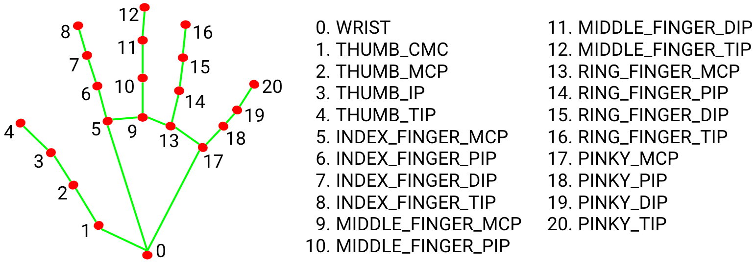
以下のコードでresults_handsに取得したlandmaksと結線をimage_blankに重畳描画しているのが分かります。
results_hands = hands.process(image)
if results_hands.multi_hand_landmarks:
        for hand_landmarks in results_hands.multi_hand_landmarks:
            #print('Handedness:', results.multi_handedness)
            mp_drawing.draw_landmarks(image_blank, hand_landmarks, mp_hands.HAND_CONNECTIONS)
アニメーションは以下のコードで実施しています。
handsは手が映っていないとき中断するので、コマ落ちしています。
そこで、コマ落ちした画像ファイルを飛ばせるように以下のように例外処理をしていますが、コマ落ちがたくさんあるので、s0という変数で中断している番号を飛ばすようにしました。
※このアニメーションではたまたま100(100個コマ落ち)でうまく描画できました
この書き方は最初は一つずつfor文をいくつも記載していたのですが、それだと中断コマ数をデータから見出す手間(これは毎回異なる)、その度に一つfor文が増えるのでやっていて収束が見えません。そこで、それをfor文で外側で回し始めて、最終的に以下のコードにたどり着いたものです。
つまり、当初設計したわけではなく、コード回しながらたどり着いた設計です。
ここまで来ると最初から以下のコードでs0を適当に選んで実行して例外出力見てこの値を調整できることが分かります。
animation
import numpy as np
import PIL.Image

s=583
images = []
s1=1
s0 =100
sk = 0
for j in range(0,s0,1):
    try:
        for i in range(s1,s,2):
            im = PIL.Image.open('./image/blank/facehands/image'+str(i)+'.png')
            im =im.resize(size=(640, 480), resample=PIL.Image.NEAREST)
            images.append(im)
    except Exception as e:
        s1=i+1
        sk += 1
        print(sk, e)
print("finish", s)
images[0].save('./image/blank/facehands.gif', save_all=True, append_images=images[1:s], duration=100*1, loop=0)
landmarkデータをcsvに吐き出すためのコード
    with open('./hands/sample_hands.csv',  'a', newline='') as f:
        landmark_point = []
        writer = csv.writer(f)
        if results.multi_hand_landmarks:
            idx += 1
            print('Handedness:', results.multi_handedness)
            for hand_landmarks in results.multi_hand_landmarks:
                for index, landmark in enumerate(hand_landmarks.landmark):
                    landmark_x = min(int(landmark.x * image_width), image_width - 1)
                    landmark_y = min(int(landmark.y * image_height), image_height - 1)

                    landmark_ = landmark_x,landmark_y
                    landmark_point.append(landmark_x)
                    landmark_point.append(landmark_y)

                    print(landmark_point)
                writer.writerow(np.array(landmark_point))
    with open('./hands/sample_hands8.csv',  'a', newline='') as f:
        landmark_point = []
        writer = csv.writer(f)
次は、landmarkが取得できていたら、位置情報を座標(整数値)に変換して1セットのlandmark_pointを取得します。
※このコードは上記参考②のリンク先のコードを参考にさせていただきました
※実際には、左右の手の座標が得られる場合がありますが、今回は右手情報は保存後削除して、左手だけを採用することとしました
※ここも改善できますが(右手左手情報が取得できている)、グーチョキパーではどちらかの手が必要ということで簡単に上の対処のままとしています
1セット(1,21,2)のlandmark_pointを取得出来たらwriter.writerowで書込みます。
※上にも書きましたが、1回でデータが二個取れたときは、一行に二個出現します。
        if results.multi_hand_landmarks:
            idx += 1
            #print('Handedness:', results.multi_handedness)
            for hand_landmarks in results.multi_hand_landmarks:
                for index, landmark in enumerate(hand_landmarks.landmark):
                    landmark_x = min(int(landmark.x * image_width), image_width - 1)
                    landmark_y = min(int(landmark.y * image_height), image_height - 1)
                    landmark_ = landmark_x,landmark_y
                    landmark_point.append(landmark_x)
                    landmark_point.append(landmark_y)
                writer.writerow(np.array(landmark_point))
残りは、画面にcv2.imshowし、ファイル保存します。
ミラー画像がいいか、まんまがいいかは好みだと思います。
※データをよく見ると右手左手は必ずしも保存の左右と一致していないので、削除は注意が必要です
※以下では、左手のみで学習データを保存することとします
データ取得時のコード全体
import mediapipe as mp
from PIL import Image
import cv2
import csv
import numpy as np

mp_drawing = mp.solutions.drawing_utils
mp_hands = mp.solutions.hands

hands = mp_hands.Hands(
    min_detection_confidence=0.7,
    min_tracking_confidence=0.5,
)
idx = 0
cap = cv2.VideoCapture(0)
while cap.isOpened():
    success, image = cap.read()
    if not success:
        print("Ignoring empty camera frame.")
        # If loading a video, use 'break' instead of 'continue'.
        continue

    # Flip the image horizontally for a later selfie-view display, and convert
    # the BGR image to RGB.
    image = cv2.cvtColor(cv2.flip(image, 1), cv2.COLOR_BGR2RGB)
    # To improve performance, optionally mark the image as not writeable to
    # pass by reference.
    image.flags.writeable = False
    results = hands.process(image)

    # Draw the hand annotations on the image.
    image.flags.writeable = True
    image = cv2.cvtColor(image, cv2.COLOR_RGB2BGR)
    image_width, image_height = image.shape[1], image.shape[0]
    with open('./hands/sample_hands6.csv',  'a', newline='') as f:
        list_landmarks = []
        landmark_point = []
        writer = csv.writer(f)
        if results.multi_hand_landmarks:
            idx += 1
            print('Handedness:', results.multi_handedness)
            for hand_landmarks in results.multi_hand_landmarks:
                for index, landmark in enumerate(hand_landmarks.landmark):
                    landmark_x = min(int(landmark.x * image_width), image_width - 1)
                    landmark_y = min(int(landmark.y * image_height), image_height - 1)

                    landmark_ = landmark_x,landmark_y #[idx,index, np.array((landmark_x, landmark_y))]
                    landmark_point.append(landmark_x)
                    landmark_point.append(landmark_y)

                    print(landmark_point)
                writer.writerow(np.array(landmark_point))
                mp_drawing.draw_landmarks(image, hand_landmarks, mp_hands.HAND_CONNECTIONS)

            cv2.imshow('MediaPipe Hands', image)
            #cv2.imwrite('./image/annotated_image' + str(idx) + '.png', cv2.flip(image, 1))
            cv2.imwrite('./image/annotated_image' + str(idx) + '.png', image)
    if cv2.waitKey(5) & 0xFF == 27:
        break
hands.close()
cap.release()
cos類似度の計算するためのコード
import numpy as np
import pandas as pd
import matplotlib.pyplot as plt

def cos_sim(v1, v2):
    return np.dot(v1, v2) / (np.linalg.norm(v1) * np.linalg.norm(v2))

df = pd.read_csv('./hands/sample_hands9.csv', sep=',')
# print(df.head(3)) #データの確認
df = df.astype(int)

print(df.iloc[0, :])

# 以下のfor文で原点0(df.iloc[i,0], df.iloc[i,1])からの座標とするかどうかを決めている
for i in range(1,len(df),1):
    for j in range(0,21,2):
        df.iloc[i,2*j+1] = df.iloc[i,2*j+1]-df.iloc[i,1]
        df.iloc[i,2*j] = df.iloc[i,2*j]-df.iloc[i,0]

cs_sim =[]
for i in range(1,len(df),1):
    cs= cos_sim(df.iloc[30,:], df.iloc[i,:])
    #print(df.iloc[i,:]-df.iloc[i,0])
    print('cos similarity: {}-{}'.format(30,i),cs)
    cs_sim.append(cs)

plt.figure(figsize=(12, 6))
plt.plot(cs_sim)
plt.ylim(0.9,)
plt.savefig('./hands/cos_sim_hands_plot9.png')
plt.show()
k-meansとPCAを用いたクラスタリングのコード
import pandas as pd
import matplotlib.pyplot as plt
from pandas import plotting
from sklearn.cluster import KMeans
from sklearn.decomposition import PCA

df = pd.read_csv('./hands/sample_hands9.csv', sep=',')
print(df.head(3))
df = df.astype(int)

plotting.scatter_matrix(df[df.columns[1:11]], figsize=(6,6), alpha=0.8, diagonal='kde')
plt.savefig('./hands/scatter_plot0-10.png')
plt.pause(5)
plt.close()

# この例では 3 つのグループに分割 (メルセンヌツイスターの乱数の種を 10 とする)
kmeans_model = KMeans(n_clusters=3, random_state=10).fit(df.iloc[:, :])
# 分類結果のラベルを取得する
labels = kmeans_model.labels_

# 分類結果を確認
print(len(labels),labels)

# それぞれに与える色を決める。
color_codes = {0:'#00FF00', 1:'#FF0000', 2:'#0000FF'} #,3:'#FF00FF', 4:'#00FFFF', 5:'#FFFF00', 6:'#000000'}
# サンプル毎に色を与える。
colors = [color_codes[x] for x in labels]

# 色分けした Scatter Matrix を描く。
plotting.scatter_matrix(df[df.columns[1:11]], figsize=(6,6),c=colors, diagonal='kde', alpha=0.8)   #データのプロット
plt.savefig('./hands/scatter_color_plot0-10.png')
plt.pause(1)
plt.close()

# 主成分分析の実行
pca = PCA()
pca.fit(df.iloc[:, :])
PCA(copy=True, n_components=None, whiten=False)

# データを主成分空間に写像 = 次元圧縮
feature = pca.transform(df.iloc[:, :])

# 第一主成分と第二主成分でプロットする
plt.figure(figsize=(6, 6))
for x, y, name in zip(feature[:, 0], feature[:, 1], df.iloc[:, 0]):
    plt.text(x, y, name, alpha=0.8, size=10)
plt.scatter(feature[:, 0], feature[:, 1], alpha=0.8, color=colors[:])
plt.title("Principal Component Analysis")
plt.xlabel("The first principal component score")
plt.ylabel("The second principal component score")
plt.savefig('./hands/PCA_hands_plot.png')
plt.pause(1)
plt.close()
色分けした Scatter Matrix を描く。
plotting.scatter_matrix(df[df.columns[0:10]], figsize=(6,6),c=colors, diagonal='kde', alpha=0.8)
結果;上の散布図に3色の色がついて、landmark 5までの点においても相関の違いが異なり、クラスタリングされることが分かります
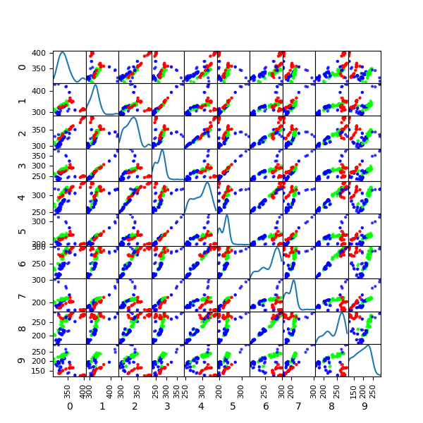
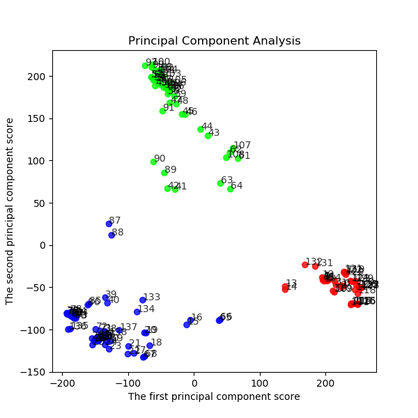
次にPCA主成分分析を行い、データを二次元に射影したのち、クラスタリングします。
結果は以下のとおり、綺麗に3つに分割されました。それぞれのクラスタの境界領域側に分布している点(14,15,64,65,88,89,132,133など)は、上記のcos-類似度のグラフの遷移領域にある点だと分かります。
因みに、青;グー、緑;チョキ、赤;パーです。
plt.scatter(feature[:, 0], feature[:, 1], alpha=0.8, color=colors)
139データのk-meansでのカテゴライズは以下の結果となっています。
139
[1 1 1 1 1 1 1 1 1 1 1 1 1 1 1 2 2 2 2 2
 2 2 2 2 2 2 2 2 2 2 2 2 2 2 2 2 2 2 2 2
 2 0 0 0 0 0 0 0 0 0 0 0 0 0 0 0 0 0 0 0
 0 0 0 0 0 2 2 2 2 2 2 2 2 2 2 2 2 2 2 2
 2 2 2 2 2 2 2 2 2 0 0 0 0 0 0 0 0 0 0 0
 0 0 0 0 0 0 0 0 0 1 1 1 1 1 1 1 1 1 1 1
 1 1 1 1 1 1 1 1 1 1 1 1 1 2 2 2 2 2 2]
こうして教師無しでもグーチョキパーは分類できそうです。
※まあ、目で見れば当然ですが、。。。
最後に、次の教師あり深層学習をやるために、この分類データを42番目のデータとして、csvに追記します。
※実際には、追記ではなく再作成しています
【参考】
④PythonでCSVファイルを読み込み・書き込み(入力・出力)
k-meansに基づくタグをデータに追記するコード
import pandas as pd
import matplotlib.pyplot as plt
from pandas import plotting
from sklearn.cluster import KMeans
import csv
import numpy as np

df = pd.read_csv('./hands/sample_hands9.csv', sep=',')

# この例では 3 つのグループに分割 (メルセンヌツイスターの乱数の種を 10 とする)
kmeans_model = KMeans(n_clusters=3, random_state=10).fit(df.iloc[:, :])
# 分類結果のラベルを取得する
labels = kmeans_model.labels_

# 分類結果を確認
print(len(labels),labels)
df['42']=labels
header = ['name', 0, 1, 2, 3, 4, 5, 6, 7, 8, 9,10,11,12,13,14,15,16,17,18,19,20,21,22,23,24,25,26,27,28,29,30,31,32,33,34,35,36,37,38,39,40,41,42]

with open('./hands/sample_hands9_.csv',  'a', newline='') as f:
    writer = csv.writer(f)
    writer.writerow(header)
    for i in range(len(df)):
        writer.writerow(np.array(df.iloc[i,:]))

# 以下検証用
df_ = pd.read_csv('./hands/sample_hands9_.csv', sep=',')
print(df_.head(3))
print(df_['42'].astype(int))

plotting.scatter_matrix(df_[df_.columns[1:11]], figsize=(6,6), alpha=0.8, diagonal='kde')
plt.savefig('./hands/scatter_plot_0-10.png')
plt.pause(5)
plt.close()
データとk-meansの分類タグに基いてmatplotlibで手を描画するコード
import cv2
import csv
import numpy as np
import pandas as pd
import matplotlib.pyplot as plt

df = pd.read_csv('./hands/sample_hands9_.csv', sep=',')
# print(df.head(3))
data_num = len(df)
# print(data_num)
df = df.astype(int)

x = []
for j in range(data_num):
    x_ = []
    for i in range(0,21,1):
        x__ = [df['{}'.format(2*i)][j],df['{}'.format(2*i+1)][j]]
        x_.append(x__)
    x.append(x_)

y = df['42']
x = np.array(x)
y = np.array(y)
print(x.shape,y.shape)

fig = plt.figure()
ax = plt.axes()
while 1:
    for j in range(0,data_num):
        for i in range(20):
            plt.plot(x[j][i][0],x[j][i][1],color='black', marker='o')
        plt.text(600,-120,y[j],size=50)
        plt.xlim(700,0)
        plt.ylim(600,-200)
        plt.title(j)
        plt.pause(0.1)
        plt.savefig('./hands/draw/data_plot{}.png'.format(j))
        plt.clf()
    if cv2.waitKey(5) & 0xFF == 27:
        break
ということで、以下のようなコードに行きつけました。
ほぼ、参考⑤のとおりです。
ただし、以下のコードはどこかでこういう記述方法をしていたのを採用しています。
dataとlabelデータの返し方はDataloaderを使う上での肝です
【参考】
・Pytorchで遊ぼう【データ成形からFNNまで】
・Input numpy ndarray instead of images in a CNN
        #以下のfloat() とlong()の指定は今回の肝です
        self.data = torch.from_numpy(np.array(x)).float()
        self.label = torch.from_numpy(np.array(y)).long()
datasetは、ほぼ上で利用して来たcsvの読込を利用しています。
transformは今回は明示的には定義していません。
HandsDatasetのコード
class HandsDataset(torch.utils.data.Dataset):
    def __init__(self, data_num, transform=None):
        self.transform = transform
        self.data_num = data_num
        self.data = []
        self.label = []
        df = pd.read_csv('./hands/sample_hands7.csv', sep=',')
        print(df.head(3)) #データの確認
        df = df.astype(int)
        x = []
        for j in range(self.data_num):
            x_ = []
            for i in range(0,21,1):
                x__ = [df['{}'.format(2*i)][j],df['{}'.format(2*i+1)][j]]
                x_.append(x__)
            x.append(x_)
        y = df['42'][:self.data_num]

        #以下のfloat() とlong()の指定は今回の肝です
        self.data = torch.from_numpy(np.array(x)).float()
        print(self.data)
        self.label = torch.from_numpy(np.array(y)).long()
        print(self.label)

    def __len__(self):
        return self.data_num

    def __getitem__(self, idx):
        out_data = self.data[idx]
        out_label =  self.label[idx]
        if self.transform:
            out_data = self.transform(out_data)
        return out_data, out_label
上のdatasetを利用するためのNetwork LitHandsのコード
class LitHands(pl.LightningModule):

    def __init__(self, hidden_size=10, learning_rate=2e-4):
        super().__init__()
        ...
        # Hardcode some dataset specific attributes
        self.num_classes = 3
        self.dims = (1, 21, 2)
        channels, width, height = self.dims
        ...

    def forward(self, x):
        ...
        return F.log_softmax(x, dim=1)

    def training_step(self, batch, batch_idx):
        ...
        return loss

    def validation_step(self, batch, batch_idx):
        ...
        return loss

    def test_step(self, batch, batch_idx):
        ...
    def configure_optimizers(self):
        ...

    def setup(self, stage=None):
        data_num=1350 #292
        self.dataset = HandsDataset(data_num, transform=None)
        n_train = int(len(self.dataset)*0.5)
        n_val = int(len(self.dataset)*0.3)
        n_test = len(self.dataset)-n_train-n_val
        print("n_train, n_val, n_test ",n_train, n_val, n_test)

        self.train_data, self.val_data, self.test_data = random_split(self.dataset,[n_train, n_val, n_test])
        print('type(train_data)',type(self.train_data))

    def train_dataloader(self):
        self.trainloader = DataLoader(self.train_data, shuffle=True, drop_last = True, batch_size=32, num_workers=0)
        return self.trainloader

    def val_dataloader(self):
        return DataLoader(self.val_data, shuffle=False, batch_size=32, num_workers=0)

    def test_dataloader(self):
        return DataLoader(self.test_data, shuffle=False, batch_size=32)
networkと学習
network
最後にnetworkと学習を記載します。
コードは参考②を参考に以下の通りとしました。
入力;(batch,index,(x,y))=(32,21,2)
出力class_num=3(グー、チョキ、パー);(3)
42⇒20⇒20⇒3とchを変更しています。
推論の最後の出力;F.log_softmax(x, dim=1)
としています。
training_stepでは、loss = F.nll_loss(logits, y)として、これを小さくするように学習します。
logitsが推論されたchでyが教師データのchです。
※今回はカテゴライズなので、MNISTなどのカテゴライズと同じF.nll_lossを利用しています。
nll_lossについては、参考⑤で考察されています。
因みに、nll_lossは、Negative Log-Likelihood (NLL) loss(負対数尤度損失)ということですね。
参考⑥⑦に詳細が解説されています。
【参考】
⑥pytorch の NLLLoss の挙動
⑦Understanding softmax and the negative log-likelihood
また、validation_stepでは、predsと正解yとの間の、acc = accuracy(preds, y)を定義して、これで精度を見ています。
客観的な精度を見るためにtest_stepを用意しました。
configure_optimizers(self)では、いつものようにAdamを利用することとしました。
データが少ないので、学習率Ir=2e-4は固定としています。
上のdatasetを利用するためのNetwork LitHandsのコード
class LitHands(pl.LightningModule):
    def __init__(self, hidden_size=10, learning_rate=2e-4):
        super().__init__()
        # Set our init args as class attributes

        self.hidden_size = hidden_size
        self.learning_rate = learning_rate

        # Hardcode some dataset specific attributes
        self.num_classes = 3
        self.dims = (1, 21, 2)
        channels, width, height = self.dims

        # Define PyTorch model
        self.model = nn.Sequential(
            nn.Flatten(),
            nn.Linear(channels * width * height, 2*hidden_size),
            nn.ReLU(),
            #nn.Dropout(0.1),
            nn.Linear(2*hidden_size, 2*hidden_size),
            nn.ReLU(),
            #nn.Dropout(0.1),
            nn.Linear(2*hidden_size, self.num_classes)
        )

    def forward(self, x):
        x = self.model(x)
        return F.log_softmax(x, dim=1)

    def training_step(self, batch, batch_idx):
        x, y = batch
        logits = self(x)
        loss = F.nll_loss(logits, y)
        #print(logits,y)
        return loss

    def validation_step(self, batch, batch_idx):
        x, y = batch
        logits = self(x)
        loss = F.nll_loss(logits, y)
        preds = torch.argmax(logits, dim=1)
        acc = accuracy(preds, y)

        # Calling self.log will surface up scalars for you in TensorBoard
        self.log('val_loss', loss, prog_bar=True)
        self.log('val_acc', acc, prog_bar=True)
        return loss

    def test_step(self, batch, batch_idx):
        # Here we just reuse the validation_step for testing
        return self.validation_step(batch, batch_idx)

    def configure_optimizers(self):
        optimizer = torch.optim.Adam(self.parameters(), lr=self.learning_rate)
        return optimizer
上のNetwork LitHandsを利用して学習するためのコード
def main():
    model = LitHands()
    print(model)
    trainer = pl.Trainer(max_epochs=2000) #収束は速い
    #trainer = pl.Trainer(max_epochs=1, gpus=1) #データ多くなったら使うかな
    trainer.fit(model) #, DataLoader(train, batch_size = 32, shuffle= True), DataLoader(val, batch_size = 32))
    trainer.test(model)
    print('training_finished')
    PATH = "hands_mlp.ckpt"
    trainer.save_checkpoint(PATH) #学習結果を保存

    pretrained_model = model.load_from_checkpoint(PATH)  #pretrainedな重みを読み込む;今は今学習した重み
    pretrained_model.freeze()
    pretrained_model.eval()

    a =  torch.tensor([[315., 420.],  #試しに出力
            [409., 401.],
            [485., 349.],
            [534., 302.],
            [574., 279.],
            [418., 205.],
            [442., 126.],
            [462.,  74.],
            [477.,  33.],
            [364., 186.],
            [370.,  89.],
            [379.,  22.],
            [386., -33.],
            [312., 192.],
            [311.,  98.],
            [316.,  37.],
            [321.,  -9.],
            [259., 218.],
            [230., 154.],
            [215., 113.],
            [204.,  77.]])
    print(a[:])
    results = pretrained_model(a[:].reshape(1,21,2))
    print(results)
    preds = torch.argmax(results)
    print(preds)

    df = pd.read_csv('./hands/sample_hands7.csv', sep=',') #教師データとは異なる適当なデータを用意
    print(df.head(3)) #データの確認
    df = df.astype(int)
    data_num = len(df)
    x = []
    for j in range(data_num):
        x_ = []
        for i in range(0,21,1):
            x__ = [df['{}'.format(2*i)][j],df['{}'.format(2*i+1)][j]]
            x_.append(x__)
        x.append(x_)
    data_ = torch.from_numpy(np.array(x)).float()
    y = df['42'][:data_num]
    label_ = torch.from_numpy(np.array(y)).long()
    count = 0
    for j in range(data_num):
        a = data_[j] #全データに対して計算
        results =  pretrained_model(a[:].reshape(1,21,2)) #全データに対して予測値計算
        preds = torch.argmax(results)
        print(j,preds,label_[j]) #予測値predsと本来の値labelと表示
        if preds== label_[j]:
            count += 1
    acc=count/data_num
    print("acc = ",acc)

if __name__ == '__main__':
    start_time = time.time()
    main()
    print('elapsed time: {:.3f} [sec]'.format(time.time() - start_time))
実行結果は以下のようになりました。
LitHandsのコード;実行結果
>python mediapipe_mlp_last.py
LitHands(
  (model): Sequential(
    (0): Flatten(start_dim=1, end_dim=-1)
    (1): Linear(in_features=42, out_features=20, bias=True)
    (2): ReLU()
    (3): Linear(in_features=20, out_features=20, bias=True)
    (4): ReLU()
    (5): Linear(in_features=20, out_features=3, bias=True)
  )
)
GPU available: True, used: False
TPU available: None, using: 0 TPU cores
...
n_train, n_val, n_test  675 405 270
type(train_data) <class 'torch.utils.data.dataset.Subset'>
...
  | Name  | Type       | Params
-------------------------------------
0 | model | Sequential | 1.3 K
-------------------------------------
1.3 K     Trainable params
0         Non-trainable params
1.3 K     Total params
Epoch 1999: 100%|██████████████████████████████████████████████████████████████████████████████████████████████████████| 34/34 [00:00<00:00, 558.63it/s, loss=0.00861, v_num=449, val_loss=0.184, val_acc=0.983]
...
Testing: 100%|██████████████████████████████████████████████████████████████████████████████████████████████████████████████████████████████████████████████████████████████████| 9/9 [00:00<00:00, 1128.01it/s]
--------------------------------------------------------------------------------
DATALOADER:0 TEST RESULTS
{'val_acc': tensor(1.), 'val_loss': tensor(0.0014)}
--------------------------------------------------------------------------------
training_finished

acc =  0.9911176905995559
elapsed time: 128.257 [sec]
pretrained_model = model.load_from_checkpoint(PATH)
print(pretrained_model)
pretrained_model.eval()
pretrained_model.freeze()
preds = pretrained_model(X) #このコードはループ内でwebcameraでxを取得したときに実施
2.予測は以下のコードで実施
要点は、datasetと同じようにa = torch.from_numpy(a).float()で予測しますが、複数データの場合があるので、a = a[:42]でデータセットを1セットに制限します。あとは、predsを計算しています。
a = np.array(landmark_point).astype(int)
a = torch.from_numpy(a).float()
# print(a.reshape(1,21,2))
a = a[:42]
results_ = pretrained_model(a[:].reshape(1,21,2))
print(results_)
preds = torch.argmax(results_)
3.画像格納をDirを分けています。ミスを見つけ易いです
グー・チョキ・パーリアルタイム予測表示
import mediapipe as mp
from PIL import Image
import cv2
import csv
import numpy as np
import torch

from mediapipe_mlp_last import LitHands

mp_drawing = mp.solutions.drawing_utils
mp_hands = mp.solutions.hands

hands = mp_hands.Hands(
    min_detection_confidence=0.7,
    min_tracking_confidence=0.5,
)

model = LitHands()
PATH = "hands_mlp.ckpt"
pretrained_model = model.load_from_checkpoint(PATH)
print(pretrained_model)
pretrained_model.eval()
pretrained_model.freeze()

image0 = cv2.imread('blank.jpg') #白紙を台紙にします

idx = 0
cap = cv2.VideoCapture(0)
while cap.isOpened():
    success, image = cap.read()
    image_blank = image0.copy() #白紙を台紙にします
    cv2.imwrite('./image/x/image_o' + str(idx) + '.png', image)
    if not success:
        print("Ignoring empty camera frame.")
        # If loading a video, use 'break' instead of 'continue'.
        continue

    # Flip the image horizontally for a later selfie-view display, and convert
    # the BGR image to RGB.
    image = cv2.cvtColor(cv2.flip(image, 1), cv2.COLOR_BGR2RGB)
    # To improve performance, optionally mark the image as not writeable to
    # pass by reference.
    image.flags.writeable = False
    results = hands.process(image)

    # Draw the hand annotations on the image.
    image.flags.writeable = True
    image = cv2.cvtColor(image, cv2.COLOR_RGB2BGR)
    image_width, image_height = image.shape[1], image.shape[0]
    with open('./hands/sample_hands8.csv',  'a', newline='') as f:
        list_landmarks = []
        landmark_point = []
        writer = csv.writer(f)
        if results.multi_hand_landmarks:
            idx += 1
            #print('Handedness:', results.multi_handedness)
            for hand_landmarks in results.multi_hand_landmarks:
                for index, landmark in enumerate(hand_landmarks.landmark):
                    landmark_x = min(int(landmark.x * image_width), image_width - 1)
                    landmark_y = min(int(landmark.y * image_height), image_height - 1)

                    landmark_ = landmark_x,landmark_y
                    landmark_point.append(landmark_x)
                    landmark_point.append(landmark_y)

                #print(landmark_point)
                a = np.array(landmark_point).astype(int)
                a = torch.from_numpy(a).float()
                #print(a.reshape(1,21,2))
                a = a[:42]
                results_ = pretrained_model(a[:].reshape(1,21,2))
                print(results_)
                preds = torch.argmax(results_)
                print(preds)
                landmark_point.append(preds)
                writer.writerow(np.array(landmark_point))

            mp_drawing.draw_landmarks(image_blank, hand_landmarks, mp_hands.HAND_CONNECTIONS)

            cv2.imshow('MediaPipe Hands_{}'.format(preds), image_blank)
            cv2.imwrite('./'+'image/{}'.format(preds) +'/image{}_'.format(preds) + str(idx) + '.png', cv2.flip(image_blank, 1))

    if cv2.waitKey(5) & 0xFF == 27:
        break
hands.close()
cap.release()
元画像
学習結果のプロット(容量の関係で偶数番号間引き)
少し苦労したので、コード載せておきます。
※学習結果のプロットのアニメ表示はコメントアウトを外して、こちらを生かします
アニメーションのためのコード
import os
import pickle
import numpy as np
import PIL.Image
import pandas as pd

df = pd.read_csv('./hands/sample_hands_results_.csv', sep=',')
print(df.head(3))
df = df.astype(int)
print(df['name'], df['42'])

s=len(df) #139 #583
images = []
s1=1
s0 =3 #100
sk=0
for j in range(0,s0,1):
    try:
        for i in range(s1,s,2):
            im = PIL.Image.open('./image/{}'.format(df['42'][i])+'/image{}_'.format(df['42'][i])+str(df['name'][i])+'.png')
            #im = PIL.Image.open('./hands/draw_results/data_plot'+str(i)+'.png')
            im =im.resize(size=(640, 478), resample=PIL.Image.NEAREST)
            images.append(im)
    except Exception as e:
        s1=i+1
        sk += 1
        print(sk,e)

print("finish", s, len(images))

images[0].save('./hands/hands_results_.gif', save_all=True, append_images=images[1:s], duration=100*1, loop=0)
matplotlibで結果のcsvデータをプロット表示するコード
import cv2
import csv
import numpy as np
import pandas as pd
import matplotlib.pyplot as plt

df = pd.read_csv('./hands/sample_hands_results_.csv', sep=',')
print(df.head(3))
data_num = len(df)
print(data_num)
df = df.astype(int)

x = []
for j in range(data_num):
    x_ = []
    for i in range(0,21,1):
        x__ = [df['{}'.format(2*i)][j],df['{}'.format(2*i+1)][j]]
        x_.append(x__)
    x.append(x_)

y = df['42']
x = np.array(x)
y = np.array(y)
print(x.shape,y.shape)

fig = plt.figure()
ax = plt.axes()
while 1:
    for j in range(0,data_num):
        for i in range(20):
            plt.plot(x[j][i][0],x[j][i][1],color='black', marker='o')
        plt.text(600,-120,y[j],size=50)
        plt.xlim(700,0)
        plt.ylim(600,-200)
        plt.title(j)
        plt.pause(0.1)
        plt.savefig('./hands/draw_results/data_plot{}.png'.format(j))
        plt.clf()
    if cv2.waitKey(5) & 0xFF == 27:
        break
・face_meshから、実際の顔へのマッピング(変換)をやりたい