分散共分散行列を特徴量として,オブジェクト検出 (object detection) やテクスチャ分類 (texture classification) のようなコンピュータビジョン分野の課題に取り組むという論文「Region Covariance: A fast descriptor for detection and classification1」 のまとめとオブジェクト検出の簡単な Python での実装.
Introduction
検出や分類問題において,特徴量選択は非常に重要である.実際,RGB 値や輝度値,その勾配などがコンピュータビジョン分野ではよく用いられているが,これらの特徴量は照明の当たり具合に頑健でなく,画像サイズによっては高次元な特徴量になってしまうなどの問題点がある.また,画像のヒストグラムを用いる手法も存在するが,ヒストグラムのビンの数を $b$,特徴量の数を $d$ とすると,ヒストグラムの次元は $b^d$ となり,特徴量の数について指数的に次元が増加してしまう.以下は RGB 値を特徴量とした $b=4, d=3$ の例.
 →
→  →
→ 
そこで,この論文では画像の領域属性 (region descriptor) として分散共分散行列を用いることを提案している.特徴量の数 $d$ に対して,分散共分散行列の次元は $d\times d$ となり,特徴量をそのまま用いたりヒストグラムを用いる場合に対し次元が小さいという利点がある.また,この論文では,分散共分散行列を用いた最近傍探索アルゴリズム (nearest neighbor search algorithm) を提案している.
Covariance as a Region Descriptor
$I$ を $W\times H$ の輝度値画像,または $W\times H\times 3$ の RGB 画像とする.この画像から得られる $W\times H\times d$ 次元の特徴量画像 $F$ を
F(x, y) = \phi(I, x, y)
とする.ここで,関数 $\phi$ は輝度値や RGB 値,勾配のようなフィルター応答などによる写像とする.矩形領域 $R\subset F$ 内の $d$ 次元特徴量ベクトルを $z_1,\dots,z_n$ とし,領域 $R$ を表現する分散共分散行列 $C_R$ を
C_R = \frac{1}{n-1}\sum_{k=1}^n(z_k - \mu)(z_k - \mu)^\top,\quad \mu=\frac1n\sum_{k=1}^n z_k
で計算する.
先述のとおり,分散共分散行列の次元は $d\times d$ であり,対称行列であることから $\frac12d(d+1)$ 個の異なる値を持つ.これは,特徴量をそのまま用いる場合 ($n\times d$ 次元) やヒストグラムを用いる場合 ($b^d$ 次元) と比べ低次元である.
また,$C_R$ は特徴点の順番や数の情報を持たないため,行列を構成する特徴量によっては回転やスケールに対して不変 (invariant) な属性となる.(例えば,$x,y$ 方向の勾配情報を用いると回転不変性は失われる)
Distance Calculation on Covariance Matrices
分散共分散行列はユークリッド空間でなく正定値対称行列の集合
\mathcal{P}(d) := \left\{X\in\mathbb{R}^{d\times d}\mid X=X^\top,X\succ O\right\}
に属している.このことは,分散共分散行列 $C_R$ について,$-C_R$ が分散共分散行列となり得ないことから確認できる.よって,分散共分散行列を用いて最近傍探索を行う際には,ユークリッド距離でなく $\mathcal{P}(d)$ 上での距離 (リー群とかリーマン多様体とかに関係する)
\rho(C_1, C_2) = \sqrt{\sum_{i=1}^d \ln^2\lambda_i(C_1, C_2)} \tag{1}
を使用する.ここで,$\lambda_i(C_1, C_2)$ は $C_1, C_2$ の一般化固有値であり,一般化固有ベクトル $x_i\neq0$ に対し
\lambda_i C_1 x_i - C_2 x_i = 0, \quad i=1, \dots, d
をみたす.
Integral Images for Fast Covariance Computation
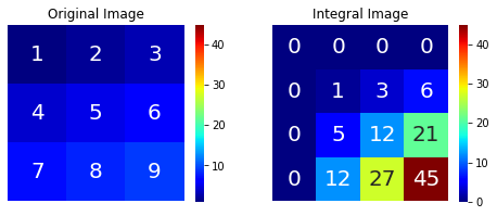
高速に分散共分散行列を計算するために,積分画像 (integral image) を使用する.積分画像とは
\text{Integral Image }(x', y') = \sum_{x<x' ,y<y'}I(x, y)
で定義される,注目ピクセルより左上に存在するピクセル値の和である.
分散共分散行列の $(i,j)$ 成分は
\begin{align}
C_R(i, j) &= \frac{1}{n-1}\sum_{k=1}^n (z_k(i) - \mu(i))(z_k(j) - \mu(j))\\
&= \frac{1}{n-1}\left[\sum_{k=1}^n z_k(i)z_k(j) - \mu(i)\sum_{k=1}^n z_k(j) - \mu(j)\sum_{k=1}^n z_k(i) + n\mu(i)\mu(j)\right]\\
&= \frac{1}{n-1}\left[\sum_{k=1}^n z_k(i)z_k(j) - \frac1n\sum_{k=1}^n z_k(i)\sum_{k=1}^n z_k(j)\right]\\
\end{align}
で計算され,$z_k$ の 1 次,2 次の和が必要なことがわかる.そこで,$W\times H\times d$ 次元の積分画像 $P$ と $W\times H\times d\times d$ 次元の積分画像 $Q$ をそれぞれ
\begin{align}
P(x',y',i) &= \sum_{x<x', y<y'}F(x, y, i), \quad i=1, \dots, d \tag{2}\\
Q(x',y',i, j) &= \sum_{x<x', y<y'}F(x, y, i)F(x, y, j), \quad i, j=1, \dots, d \tag{3}
\end{align}
で定義する.また,1 点 $(x, y)$ における積分画像の値をそれぞれ
\begin{align}
p_{x, y} &= \left[P(x, y, 1), \dots, P(x, y, d)\right]^\top\\
Q_{x, y} &=
\begin{pmatrix}
Q(x, y, 1, 1) & \cdots & Q(x, y, 1, d)\\
\vdots & \ddots & \vdots\\
Q(x, y, d, 1) & \cdots & Q(x, y, d, d)
\end{pmatrix}
\end{align}
とする.
左上が $(x',y')$,右下が $(x'', y'')$ の矩形領域を $R(x', y'; x'', y'')$ とするとき,この矩形領域における分散共分散行列は,$n = (x'' - x')\cdot(y'' - y')$ として,
\begin{align}
C_{R(x', y'; x'', y'')} = \frac{1}{n-1}\left[Q_{x'', y''} + Q_{x', y'} - Q_{x'', y'} - Q_{x', y''}\\
-\frac1n(p_{x'', y''} + p_{x', y'} - p_{x'', y'} - p_{x', y''})(p_{x'', y''} + p_{x', y'} - p_{x'', y'} - p_{x', y''})^\top\right] \tag{4}
\end{align}
で計算できる.

Object Detection
この論文では画像の特徴量としてピクセルの $x, y$ 座標,画像の RGB 値 $R(x, y), G(x, y), B(x, y)$,画像の輝度値 $I(x, y)$ の 1 次と 2 次の勾配の絶対値の 9 つを用い,オブジェクト検出を行なっている.なお 1 次と 2 次の勾配はフィルター $[-1, 0, 1],[-1, 2, -1]$ を用いて計算される.
F(x, y) = \left[x, y, R(x, y), G(x, y), B(x, y), \left|\frac{\partial I(x, y)}{\partial x}\right|, \left|\frac{\partial I(x, y)}{\partial y}\right|, \left|\frac{\partial^2 I(x, y)}{\partial x^2}\right|, \left|\frac{\partial^2 I(x, y)}{\partial y^2}\right|\right]^\top \tag{5}
オブジェクト検出の手順
- 入力画像から分散共分散行列を (4) 式により計算する.
- ターゲット画像に対し,9 種類のウィンドウサイズとステップサイズを用いて力任せ探索 (brute force search) を行い,各ウィンドウについて分散共分散行列を計算する.
- (1) 式で計算される分散共分散行列間の距離が小さいウィンドウを検出する.
論文中では,オブジェクトを表現するのに 5 つの分散共分散行列を作り,分散共分散行列間の距離が小さい 1000 個のウィンドウについて,再度 5 つの分散共分散行列の計算を行なっているが,簡単のため 1 つのみで数値実験を行なった.
数値実験
左の画像のピンクで囲んだ箇所を入力画像とし,解像度の異なる右の 2 枚の画像に対しオブジェクト検出を行なった.

ソースコードと簡単な解説
ソースコードは以下の通り,実行したノートブックは Github に.
- 関数
calc_distanceで (1) 式の距離の計算を行なう.一般化固有値はscipy.linalg.eighというエルミート行列用の固有値計算関数を使用した. - 関数
_extract_featuresで (5) 式の特徴量を抽出する.cv2.filter2Dを用いて勾配計算を行なっている. - 関数
_calc_integral_imagesで (2), (3) 式の積分画像を計算する.積分画像はcv2.integralで計算している. - 関数
_calc_covarianceで (4) 式の計算を行なっている.
from typing import List, Tuple
from itertools import product

import cv2
import numpy as np
from scipy.linalg import eigh
from tqdm import tqdm


def calc_distance(x: np.ndarray, y: np.ndarray) -> float:
    w = eigh(x, y, eigvals_only=True)
    return np.linalg.norm(np.log(w) ** 2)


class RegionCovarianceDetector:
    """
    Object Detector Using Region Covariance

    Parameters
    ----------
    coord : bool, optional (default=True)
        Whether use coordinates as features or not.

    color : bool, optional (default=True)
        Whether use color channels as features or not.

    intensity : bool, optional (default=False)
        Whether use intensity as feature or not.

    kernels : a list of np.ndarray, optional (default=None)
        Filters applied to intensity image. If None, no filters are used.

    ratio : float, optional (default=1.15)
        Scaling factor between two consecutive scales of the search window size and step size.

    step : int, optional (default=3)
        The minimum step size.

    n_windows : int, optional (default=9)
        The number of scales of the windows.

    eps : float, optional (default=1e-16)
        Small number to keep covariance matrices in SPD.

    Attributes
    ----------
    object_shape_ : (int, int)
        The object's shape.

    object_covariance_ : np.ndarray, shape (n_features, n_features)
        Covariance matrix of the object.
    """

    def __init__(
            self,
            coord: bool = True,
            color: bool = True,
            intensity: bool = False,
            kernels: List[np.ndarray] = None,
            ratio: float = 1.15,
            step: int = 3,
            n_windows: int = 9,
            eps: float = 1e-16
    ):
        self.coord = coord
        self.color = color
        self.intensity = intensity
        self.kernels = kernels
        self.ratio = ratio
        self.step = step
        self.n_windows = n_windows
        self.eps = eps

        self.object_shape_ = None
        self.object_covariance_ = None

    def _extract_features(self, img: np.ndarray) -> List[np.ndarray]:
        """
        Extract image features.

        Parameters
        ----------
        img : np.ndarray, shape (h, w, c)
            uint8 RGB image

        Returns
        -------
        features : a list of np.ndarray
            Features such as intensity, its gradient and so on.
        """
        h, w, c = img.shape[:3]
        intensity = cv2.cvtColor(img, cv2.COLOR_BGR2HSV)[:, :, 2] / 255.
        features = list()

        # use coordinates
        if self.coord:
            features.append(np.tile(np.arange(w, dtype=float), (h, 1)))
            features.append(np.tile(np.arange(h, dtype=float).reshape(-1, 1), (1, w)))

        # use color channels
        if self.color:
            for i in range(c):
                features.append(img[:, :, i].astype(float) / 255.)

        # use intensity
        if self.intensity:
            features.append(intensity)

        # use filtered images
        if self.kernels is not None:
            for kernel in self.kernels:
                features.append(np.abs(cv2.filter2D(intensity, cv2.CV_64F, kernel)))

        return features

    def _calc_integral_images(self, img: np.ndarray) -> Tuple[np.ndarray, np.ndarray]:
        """
        Calculate integral images.

        Parameters
        ----------
        img : np.ndarray, shape (h, w, c)
            uint8 RGB image

        Returns
        -------
        P : np.ndarray, shape (h+1, w+1, n_features)
            First order integral images of features.

        Q : np.ndarray, shape (h+1, w+1, n_features, n_features)
            Second order integral images of features.
        """
        h, w = img.shape[:2]
        features = self._extract_features(img)
        length = len(features)

        # first order integral images
        P = cv2.integral(np.array(features).transpose((1, 2, 0)))

        # second order integral images
        Q = cv2.integral(
            np.array(list(map(lambda x: x[0] * x[1], product(features, features)))).transpose((1, 2, 0))
        )
        Q = Q.reshape(h + 1, w + 1, length, length)
        return P, Q

    def _calc_covariance(self, P: np.ndarray, Q: np.ndarray, pt1: Tuple[int, int], pt2: Tuple[int, int]) -> np.ndarray:
        """
        Calculate covariance matrix from integral images.

        Parameters
        ----------
        P : np.ndarray, shape (h+1, w+1, n_features)
            First order integral images of features.

        Q : np.ndarray, shape (h+1, w+1, n_features, n_features)
            Second order integral images of features.

        pt1 : (int, int)
            Left top coordinate.

        pt2 : (int, int)
            Right bottom coordinate.

        Returns
        -------
        covariance : np.ndarray, shape (n_features, n_features)
            Covariance matrix.
        """
        x1, y1 = pt1
        x2, y2 = pt2
        q = Q[y2, x2] + Q[y1, x1] - Q[y1, x2] - Q[y2, x1]
        p = P[y2, x2] + P[y1, x1] - P[y1, x2] - P[y2, x1]
        n = (y2 - y1) * (x2 - x1)
        covariance = (q - np.outer(p, p) / n) / (n - 1) + self.eps * np.identity(P.shape[2])
        return covariance

    def fit(self, img: np.ndarray):
        """
        Calculate the object covariance matrix.

        Parameters
        ----------
        img : np.ndarray, shape (h, w, c)
            uint8 RGB image

        Returns
        -------
        : Fitted detector.
        """
        h, w = img.shape[:2]
        P, Q = self._calc_integral_images(img)

        # normalize about coordinates
        if self.coord:
            for i, size in enumerate((w, h)):
                P[:, :, i] /= size
                Q[:, :, i] /= size
                Q[:, :, :, i] /= size

        # calculate covariance matrix
        self.object_covariance_ = self._calc_covariance(P, Q, (0, 0), (w, h))
        self.object_shape_ = (h, w)
        return self

    def predict(self, img: np.ndarray) -> Tuple[Tuple[int, int], Tuple[int, int], float]:
        """
        Compute object's position in the target image.

        Parameters
        ----------
        img : np.ndarray, shape (h, w, c)
            uint8 RGB image

        Returns
        -------
        pt1 : (int, int)
            Left top coordinate.

        pt2 : (int, int)
            Right bottom coordinate.

        score : float
            Dissimilarity of object and target covariance matrices.
        """
        tar_h, tar_w = img.shape[:2]
        obj_h, obj_w = self.object_shape_
        P, Q = self._calc_integral_images(img)

        # search window's shape and step size
        end = (self.n_windows + 1) // 2
        start = end - self.n_windows
        shapes = [(int(obj_h * self.ratio ** i), int(obj_w * self.ratio ** i)) for i in range(start, end)]
        steps = [int(self.step * self.ratio ** i) for i in range(self.n_windows)]

        distances = list()
        for shape, step in tqdm(zip(shapes, steps)):
            p_h, p_w = shape
            p_P, p_Q = P.copy(), Q.copy()

            # normalize about coordinates
            if self.coord:
                for i, size in enumerate((p_w, p_h)):
                    p_P[:, :, i] /= size
                    p_Q[:, :, i] /= size
                    p_Q[:, :, :, i] /= size

            distance = list()
            y1, y2 = 0, p_h
            while y2 <= tar_h:
                dist = list()
                x1, x2 = 0, p_w
                while x2 <= tar_w:
                    # calculate covariance matrix
                    p_cov = self._calc_covariance(p_P, p_Q, (x1, y1), (x2, y2))

                    # jump horizontally
                    x1 += step
                    x2 += step

                    # calculate dissimilarity of two covariance matrices
                    dist.append(calc_distance(self.object_covariance_, p_cov))

                # jump vertically
                y1 += step
                y2 += step
                distance.append(dist)
            distances.append(np.array(distance))

        # choose the most similar window
        min_indices = list(map(np.argmin, distances))
        min_index = int(np.argmin([dist.flatten()[i] for i, dist in zip(min_indices, distances)]))
        min_step = steps[min_index]
        min_shape = shapes[min_index]
        min_indice = min_indices[min_index]
        b_h, b_w = distances[min_index].shape

        pt1 = ((min_indice % b_w) * min_step, (min_indice // b_w) * min_step)
        pt2 = (pt1[0] + min_shape[1], pt1[1] + min_shape[0])
        score = distances[min_index].flatten()[min_indice]
        return pt1, pt2, score
実行結果,計算時間はそれぞれ 6.22 s, 19.7 s.
n_windows や step の値を変えればもう少し速くできる.

-
Tuzel, O., Porikli, F., & Meer, P. (2006, May). Region covariance: A fast descriptor for detection and classification. In European conference on computer vision (pp. 589-600). Springer, Berlin, Heidelberg. ↩