次元削減や特徴量抽出の手法として有名な主成分分析 (Principal Component Analysis, PCA) とその応用 (Kernel PCA, 2DPCA1) の理論と Python での実装の比較を行なう.
主成分分析の理論
第 1 主成分
$M$ 個のデータ $a_1,\ldots,a_M\in\mathbb{R}^n$ の第 $1$ 主成分 $x_1\in\mathbb{R}^n$ は,中心化されたデータ
$$a_i - \bar{a},\quad \bar{a} = \frac1M\sum_{i=1}^M a_i$$
の分散が最大となる方向で長さ $1$ のベクトルとして求められる.
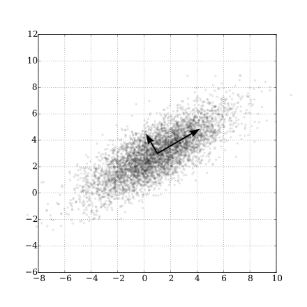
つまり,次の最大化問題の最適解と解釈できる.
\begin{align}
\max_{x\in\mathbb{R}^n} &\quad \frac1M\sum_{i=1}^M\left((a_i - \bar{a})^\top x\right)^2\\
\text{s.t.} &\quad \|x\|_2 = 1
\end{align}
ここで,データの分散共分散行列を $C := \frac1M\sum_{i=1}^M(a_i - \bar{a})(a_i - \bar{a})^\top$ とすると,
\begin{align}
\max_{x\in\mathbb{R}^n} \ \frac1M\sum_{i=1}^M\left((a_i - \bar{a})^\top x\right)^2 &= \max_{x\in\mathbb{R}^n} \ x^\top\left[\frac1M\sum_{i=1}^M(a_i - \bar{a})(a_i - \bar{a})^\top\right] x\\
&= \max_{x\in\mathbb{R}^n}\ x^\top C x
\end{align}
より,第 $1$ 主成分 $x_1$ は
x_1 = \mathop{\mathrm{arg~max}}_{x\in\mathbb{R^n}}\left\{x^\top C x \mid \|x\|_2 = 1\right\}
となり,分散共分散行列 $C$ の最大固有値に対応する固有ベクトルと一致する.
第 2 主成分
中心化されたデータ $a_i - \bar{a}$ から第 1 主成分方向を引いた上で,第 1 主成分と同様の計算を行なう.つまり,
\begin{align}
\max_{x\in\mathbb{R}^n} &\quad \frac1M\sum_{i=1}^M\left(\left(a_i - \bar{a} - \left(x_1^\top (a_i - \bar{a})\right)x_1\right)^\top x\right)^2\\
\text{s.t.} &\quad \|x\|_2 = 1
\end{align}
を扱う.ここで,
\begin{align}
a_i - \bar{a} - \left(x_1^\top (a_i - \bar{a})\right)x_1 &= a_i - \bar{a} - \left(x_1x_1^\top\right)(a_i - \bar{a})\\
&= \left(I_n - x_1x_1^\top\right)(a_i - \bar{a})
\end{align}
と式変形できる.$P_1 = I_n - x_1x_1^\top$ とし,分散共分散行列 $C$ の固有値を $\lambda_1\geq\cdots\geq\lambda_n$,対応する固有ベクトルを $v_1, \ldots, v_n$ とすると,実対称行列の固有ベクトルの直交性より,
\begin{cases}
P_1v_i = 0 & (i = 1)\\
P_1v_i = v_i & (i \neq 1)
\end{cases}
が成り立つ.また,
\begin{align}
\max_{x\in\mathbb{R}^n} \ \frac1M\sum_{i=1}^M\left(\left(a_i - \bar{a} - \left(x_1^\top (a_i - \bar{a})\right)x_1\right)^\top x\right)^2 &= \max_{x\in\mathbb{R}^n} \ \frac1M\sum_{i=1}^M\left((a_i - \bar{a})^\top P_1 x\right)^2\\
&= \max_{x\in\mathbb{R}^n}\ (P_1x)^\top C (P_1x)
\end{align}
より,第 $2$ 主成分 $x_2$ は
x_2 = \mathop{\mathrm{arg~max}}_{x\in\mathbb{R^n}}\left\{(P_1x)^\top C (P_1x) \mid \|x\|_2 = 1\right\}
となり,分散共分散行列 $C$ の 2 番目に大きい固有値 $\lambda_2$ に対応する固有ベクトルと一致する.
同様の議論より,第 $k$ 主成分 $x_k$ は $\lambda_k$ に対応する固有ベクトルと一致することがわかり,データ $a_1, \ldots, a_M$ の主成分分析は分散共分散行列 $C$ の固有値問題に帰着される.
次元削減
データ $a_1, \ldots, a_M$ から $d$ 個の主成分 $x_1, \ldots, x_d$ が得られたとき,新たなデータ $a\in\mathbb{R}^n$ の次元削減を考える.$a$ を$d$ 個の主成分の線形結合で近似することを考えると,$X_d = [x_1,\ldots,x_d]$ を用いて,
a \approx X_d y + \bar{a}
とかける.よって,主成分の直交性 $\left(X_d^\top X_d = I_d\right)$ より,
y = X_d^\top (a - \bar{a})
と $d$ 次元に次元削減することができる.
Kernel PCA の理論2
主成分
データ空間 $\mathbb{R}^n$ からある再生核ヒルベルト空間 (Reproducing Kernel Hilbert Space, RKHS) $\mathcal{H}$ への写像を $\phi$ とする.さらに,
\bar{\phi} = \frac1M \sum_{i=1}^M \phi(a_i)\\
\Phi = [\phi(a_1),\ldots, \phi(a_M)]\\
\tilde{\Phi} = \left[\phi(a_1) - \bar{\phi},\ldots, \phi(a_M) - \bar{\phi}\right]
とすると,PCA の目的関数は
\begin{align}
\frac1M\sum_{i=1}^M\left(\left(\phi(a_i) - \bar{\phi}\right)^\top x\right)^2 &= \frac1M x^\top\left[\sum_{i=1}^M\left(\phi(a_i) - \bar{\phi}\right)\left(\phi(a_i) - \bar{\phi}\right)^\top\right] x\\
&= \frac1M x^\top\tilde\Phi\tilde\Phi^\top x
\end{align}
となる.主成分分析は $\frac1M\tilde\Phi\tilde\Phi^\top$ の固有値問題に帰着されるので,
\frac1M\tilde\Phi\tilde\Phi^\top x = \lambda x
を考える.$z = \tilde\Phi^\top x$ とすると,
x = \frac1{M\lambda}\tilde\Phi z
とかける.これを固有方程式の左辺,右辺にそれぞれ代入すると,
\begin{align}
\frac1M\tilde\Phi\tilde\Phi^\top x &= \frac1M\tilde\Phi\tilde\Phi^\top\left(\frac1{M\lambda}\tilde\Phi z\right)\\
&= \frac1{M^2\lambda}\tilde\Phi\left(\tilde\Phi^\top\tilde\Phi\right)z\\
\lambda x &= \frac1M\tilde\Phi z
\end{align}
となり,
\begin{align}
\frac1{M^2\lambda}\tilde\Phi\left(\tilde\Phi^\top\tilde\Phi\right)z = \frac1M\tilde\Phi z \iff \tilde\Phi\left(\frac1M\tilde\Phi^\top\tilde\Phi\right)z = \tilde\Phi \lambda z
\end{align}
とかける.ここで,行列 $\tilde\Phi^\top\tilde\Phi\in\mathbb{R}^{M\times M}$ は,$k(a_i, a_j) = \phi(a_i)^\top\phi(a_j)$ として,
\begin{align}
\left(\tilde\Phi^\top\tilde\Phi\right)_{i,j} &= (\phi(a_i) - \bar{\phi})^\top(\phi(a_j) - \bar{\phi})\\
&= k(a_i, a_j) - \frac1M\sum_{\ell=1}^Mk(a_i, a_\ell) - \frac1M\sum_{k=1}^Mk(a_k, a_j) + \frac1{M^2}\sum_{k, \ell=1}^Mk(a_k, a_\ell)
\end{align}
より,全成分が $1$ の行列を $\mathbf{1}\in\mathbb{R}^{M\times M}$,$\Phi^\top\Phi = K$ として,
\tilde\Phi^\top\tilde\Phi = K - \frac1M K\mathbf{1} - \frac1M\mathbf{1} K+ \frac1{M^2}\mathbf{1} K \mathbf{1}
で計算される.以上より,$\frac1M\tilde\Phi\tilde\Phi^\top$ の固有値 $\lambda$ に対応する固有ベクトル $x$ は,$M$ 次元正方行列 $\frac1M\tilde\Phi^\top\tilde\Phi$ の固有値 $\lambda$ に対応する固有ベクトル $z\in\mathbb{R}^M$ を用いて,
x = \frac1{M\lambda}\tilde\Phi z
と計算される.
次元削減
データ $a_1, \ldots, a_M$ から $d$ 個の主成分 $x_1, \ldots, x_d$ が得られたとき,新たなデータ $a\in\mathbb{R}^n$ の次元削減を考える.$\phi(a)$ を$d$ 個の主成分の線形結合で近似することを考えると,$X_d = [x_1,\ldots,x_d]$ を用いて,
\phi(a) \approx X_d y + \bar{\phi}
とかける.よって,主成分の直交性 $\left(X_d^\top X_d = I_d\right)$ より,
y = X_d^\top \left(\phi(a) - \bar{\phi}\right)
と $d$ 次元に次元削減することができる.
(補足)
\left<x_i, x_j\right>_{\mathcal H} = \delta_{i, j}
と直交化する際,
\left<x_i, x_i\right>_{\mathcal H} = \frac1{M\lambda_i^2}z_i^\top \left(\frac1M\Phi^\top\Phi \right)z_i = \frac{1}{M\lambda_i}\|z_i\|_2^2 = 1
をみたすように $z_i$ は規格化される.
2DPCA の理論1
画像のような 2 次元データ $A_1, \ldots, A_M\in\mathbb{R}^{m\times n}$ が与えられたとき,PCA では$\mathbb{R}^{mn}$ 上の 1 次元ベクトルに変換して扱うのに対し,Two-Dimensional PCA (2DPCA) では 2 次元のまま扱う.
主成分
確率変数 $A\in\mathbb{R}^{m\times n}$ を $n$ 次元ベクトル $x$ により $m$ 次元に写像することを考える.つまり,
y = A x \tag{1}
により特徴量ベクトル $y\in\mathbb{R}^m$ を得ることを考える.このとき,$x$ の指標として $y$ の分散共分散行列
\begin{align}
S_x &= \mathbb{E}\left[\left(y - \mathbb{E}[y]\right)\left(y - \mathbb{E}[y]\right)^\top\right]\\
&= \mathbb{E}\left[\left(Ax - \mathbb{E}[Ax]\right)\left(Ax - \mathbb{E}[Ax]\right)^\top\right]\\
&= \mathbb{E}\left[\left(A - \mathbb{E}[A]\right)x(\left(A - \mathbb{E}[A]\right)x)^\top\right]\\
\end{align}
のトレース $\mathrm{tr},S_x$,すなわち $y$ の分散を最大化する.
\begin{align}
\mathrm{tr}\,S_x &= \mathrm{tr}\,\mathbb{E}\left[\left(A - \mathbb{E}[A]\right)x(\left(A - \mathbb{E}[A]\right)x)^\top\right]\\
&= \mathrm{tr}\,\mathbb{E}\left[x^\top\left(A - \mathbb{E}[A]\right)^\top\left(A - \mathbb{E}[A]\right)x\right]\\
&= x^\top\mathbb{E}\left[\left(A - \mathbb{E}[A]\right)^\top\left(A - \mathbb{E}[A]\right)\right]x
\end{align}
より,データ $A_1, \ldots, A_M\in\mathbb{R}^{m\times n}$ が観測されたとき,$\mathrm{tr},S_x$ は,
\bar{A} = \frac1M\sum_{i=1}^MA_i\\
G_t = \frac1M\sum_{i=1}^M\left(A_i - \bar{A}\right)^\top\left(A_i - \bar{A}\right)
を用いて
\mathrm{tr}\,S_x = x^\top G_t x
と計算でき,このとき,
x_1 = \mathop{\mathrm{arg~max}}_{x\in\mathbb{R}^n}\left\{x^\top G_t x \mid \|x\|_2 = 1\right\}
と $G_t$ の最大固有値問題に帰着する.
次元削減
データ $A_1, \ldots, A_M$ から $G_t$ の $d$ 個の固有ベクトル $x_1, \ldots, x_d$ が得られたとき,新たなデータ $A\in\mathbb{R}^{m\times n}$ の次元削減を考える.$X_d = [x_1, \ldots, x_d] \in\mathbb{R}^{n\times d}$ とすると (1) 式より
Y_d = AX_d
と $m\times d$ 次元に次元削減することができる.また,
A \approx Y_dX_d^\top
と近似的に復元される.
PCA と 2DPCA の比較表
| PCA | 2DPCA | |
|---|---|---|
| 入力次元 | $\mathbb{R}^{mn}$ | $\mathbb{R}^{m\times n}$ |
| 圧縮次元 | $\mathbb{R}^{d}$ | $\mathbb{R}^{m\times d}$ |
| 分散共分散行列の次元 | $\mathbb{R}^{mn\times mn}$ | $\mathbb{R}^{n\times n}$ |
| $X_d$ の次元 | $\mathbb{R}^{mn\times d}$ | $\mathbb{R}^{n\times d}$ |
Python での実行例
PCA と Kernel PCA は scikit-learn の実装を,2DPCA は自分で実装したものを使用した.実装したコードは最後に記載する.
データセットの準備
実行例として,28x28 の手書き数字画像データセット MNIST を使用した.次のように 0 の画像 6902 枚を学習に,0 と 1 の画像を 1 枚ずつ検証に用いた.
from sklearn import datasets
mnist = datasets.fetch_openml('mnist_784', data_home='../../data/')
mnist_data = mnist.data / 255.
mnist_0 = mnist_data[mnist.target == '0']

mnist_shape = (28, 28)
train = mnist_0[:-1]
test_0 = mnist_0[-1].reshape(1, -1)
test_1 = mnist_data[mnist.target == '1'][-1].reshape(1, -1)
PCA の学習
分散共分散行列から 5 個の固有ベクトルを学習した.KernelPCA は fit_inverse_transform=True としないと次元削減から復元ができないことに注意する.
from sklearn.decomposition import PCA, KernelPCA

n_components = 5
%time pca = PCA(n_components=n_components).fit(train)
%time kpca = KernelPCA(n_components=n_components, fit_inverse_transform=True).fit(train)
%time tdpca = TwoDimensionalPCA(n_components=n_components).fit(train.reshape(-1, *mnist_shape))
学習時間は PCA, Kernel PCA, 2DPCA の順に以下の通り.Kernel PCA が特に重いことがわかる.
CPU times: user 545 ms, sys: 93.9 ms, total: 639 ms
Wall time: 310 ms
CPU times: user 10.9 s, sys: 1.22 s, total: 12.1 s
Wall time: 7.8 s
CPU times: user 97.6 ms, sys: 59.3 ms, total: 157 ms
Wall time: 195 ms
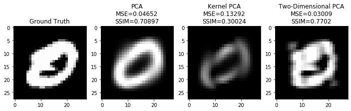
PCA による次元削減と画像の復元
transform で次元削減,inverse_transform で 0 の画像の復元を行なった.
%time pca_result_0 = pca.inverse_transform(pca.transform(test_0))
%time kpca_result_0 = kpca.inverse_transform(kpca.transform(test_0))
%time tdpca_result_0 = tdpca.inverse_transform(tdpca.transform(test_0.reshape(1, *mnist_shape)))
計算時間は PCA, Kernel PCA, 2DPCA の順に以下の通り.
CPU times: user 1.17 ms, sys: 2.72 ms, total: 3.89 ms
Wall time: 4.26 ms
CPU times: user 14.3 ms, sys: 2.24 ms, total: 16.5 ms
Wall time: 11.5 ms
CPU times: user 90 µs, sys: 3 µs, total: 93 µs
Wall time: 103 µs
復元結果
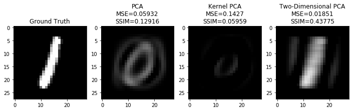
1 の画像に対しても同様に次元削減・復元を行った.
2DPCA のソースコード
実行したノートブックは Github に.
from typing import Union

import numpy as np
from scipy.linalg import eigh
from sklearn.exceptions import NotFittedError


class TwoDimensionalPCA:
    def __init__(self, n_components: Union[int, None] = None):
        self.n_components_ = n_components

        self.components_ = None
        self.mean_ = None

    def fit(self, X: np.ndarray):
        """
        Parameters
        ----------
        X : np.ndarray, shape (n_samples, height, width)
        """
        if X.ndim != 3:
            raise ValueError(f"Expected 3D array, got {X.ndim}D array instead")

        self.mean_ = np.mean(X, axis=0)
        cov = np.mean([x.T @ x for x in X - self.mean_], axis=0)
        n_features = cov.shape[0]

        if self.n_components_ is None or self.n_components_ > n_features:
            self.n_components_ = n_features
        self.components_ = eigh(cov, eigvals=(n_features - self.n_components_, n_features - 1))[1][:, ::-1]
        return self

    def transform(self, X: np.ndarray) -> np.ndarray:
        """
        Parameters
        ----------
        X : np.ndarray, shape (n_samples, height, width)

        Returns
        -------
        : np.ndarray, shape (n_samples, height, n_components)
        """
        if self.components_ is None:
            raise NotFittedError(
                "This PCA instance is not fitted yet. "
                "Call 'fit' with appropriate arguments before using this estimator.")

        if X.ndim != 3:
            raise ValueError(f"Expected 3D array, got {X.ndim}D array instead")

        return np.array([x @ self.components_ for x in X])

    def inverse_transform(self, X: np.ndarray) -> np.ndarray:
        """
        Parameters
        ----------
        X : np.ndarray, shape (n_samples, height, n_components)

        Returns
        -------
        : np.ndarray, shape (n_samples, height, width)
        """
        return np.array([x @ self.components_.T for x in X])

    def fit_transform(self, X: np.ndarray) -> np.ndarray:
        """
        Parameters
        ----------
        X : np.ndarray, shape (n_samples, height, width)

        Returns
        -------
        : np.ndarray, shape (n_samples, height, n_components)
        """
        self.fit(X)
        return self.transform(X)