はじめに

本記事は以下の人を対象としています．

筋骨格シミュレータに興味がある人
MuJoCoに興味がある人

本記事では3_Analyse_movements.ipynbをGoogle Colabで実行した際の手順と結果に関してまとめる．

MyoSuiteとは

MuJoCoを学習モジュールとして組み込んだ筋骨格シミュレータ

2024年にICRAにてworkshopを展開
https://sites.google.com/view/myosuite/myosymposium/icra24

Tutorial Notebook

実施事項

Tutorialに記載のコードを1つずつ試して, Errorになったところは都度修正版を記載する.

ライブラリのinstallと環境設定

!pip install -U myosuite
!pip install tabulate matplotlib torch gym==0.13 git+https://github.com/aravindr93/mjrl.git@pvr_beta_1vk
!pip install scikit-learn

%env MUJOCO_GL=egl

ライブラリのimportと結果表示の関数

from myosuite.utils import gym # importが上手くいくと"MyoSuite:> Registering Myo Envs"と表示される
import skvideo.io
import numpy as np
import os

from IPython.display import HTML
from base64 import b64encode

def show_video(video_path, video_width = 400):

  video_file = open(video_path, "r+b").read()

  video_url = f"data:video/mp4;base64,{b64encode(video_file).decode()}"
  return HTML(f"""<video autoplay width={video_width} controls><source src="{video_url}"></video>""")

modelのloadとpolicyの準備

# stable-baselines3のinstall
!pip install stable-baselines3

from stable_baselines3 import PPO
env = gym.make('myoElbowPose1D6MRandom-v0')

env.reset()
pi = PPO("MlpPolicy", env, verbose=0)

pi.learn(total_timesteps=1000)

stable_baselines3についてはnpakaさんの資料を参照

actionによる筋負荷データの出力

frames = []
data_store = []
for _ in range(10): # 10 episodes
    for _ in range(100): # 100 samples for each episode
        frame = env.sim.renderer.render_offscreen(
            width=400,
            height=400,
            camera_id=0
        )
        frames.append(frame)
        o = env.get_obs()
        a = pi.predict(o)[0]
        next_o, r, done, *_, ifo = env.step(a) # take a random action

        data_store.append({"action":a.copy(),
                            "jpos":env.sim.data.qpos.copy(),
                            "mlen":env.sim.data.actuator_length.copy(),
                            "act":env.sim.data.act.copy()})

env.close()

os.makedirs('videos', exist_ok=True)
# make a local copy
skvideo.io.vwrite('videos/temp.mp4', np.asarray(frames),outputdict={"-pix_fmt": "yuv420p"})
show_video('videos/temp.mp4')

残タスク

action, jpos, mlen, actがそれぞれ何を示すのか記載

出力結果

解析結果の表示

import matplotlib.pyplot as plt
from sklearn.decomposition import NMF

def VAF(W, H, A):
    """
    Args:
        W: ndarray, m x rank matrix, m-muscles x activation coefficients obtained from (# rank) nmf
        H: ndarray, rank x L matrix, basis vectors obtained from nmf where L is the length of the signal
        A: ndarray, m x L matrix, original time-invariant sEMG signal
    Returns:
        global_VAF: float, VAF calculated for the entire A based on the W&H
        local_VAF: 1D array, VAF calculated for each muscle (column) in A based on W&H
    """
    SSE_matrix = (A - np.dot(W, H))**2
    SST_matrix = (A)**2

    global_SSE = np.sum(SSE_matrix)
    global_SST = np.sum(SST_matrix)
    global_VAF = 100 * (1 - global_SSE / global_SST)

    local_SSE = np.sum(SSE_matrix, axis = 0)
    local_SST = np.sum(SST_matrix, axis = 0)
    local_VAF = 100 * (1 - np.divide(local_SSE, local_SST))

    return global_VAF, local_VAF

act = np.array([dd['act'] for dd in data_store])

VAFstore=[]
SSE, SST = [], []

sample_points = [1,2,3,4,5,10,20,30]
for isyn in sample_points:
    nmf_model = NMF(n_components=isyn, init='random', random_state=0);
    W = nmf_model.fit_transform(act)
    H = nmf_model.components_

    global_VAF, local_VAF = VAF(W, H, act)

    VAFstore.append(global_VAF)

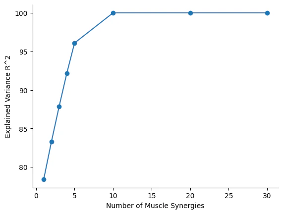
plt.plot(sample_points,VAFstore,'-o')
plt.xlabel('Number of Muscle Synergies')
plt.ylabel('Explained Variance R^2')
plt.gca().spines['top'].set_visible(False)
plt.gca().spines['right'].set_visible(False)

sample_pointsはNon-negative Matrix Factorization(NMF)実行時の次元数
- 一応>1000でも実行はできる
Muscle Synergyとは筋グループの数
- sample_pointsの値が増えるということは筋グループの数が増えるということ
- 今回だとMuscle Synergyは10未満が適度に分解されていい値？