Introduction
I am writing a post about how to create Excel report with Sharperlight Excel Add-in here.
Creating a Report in Excel
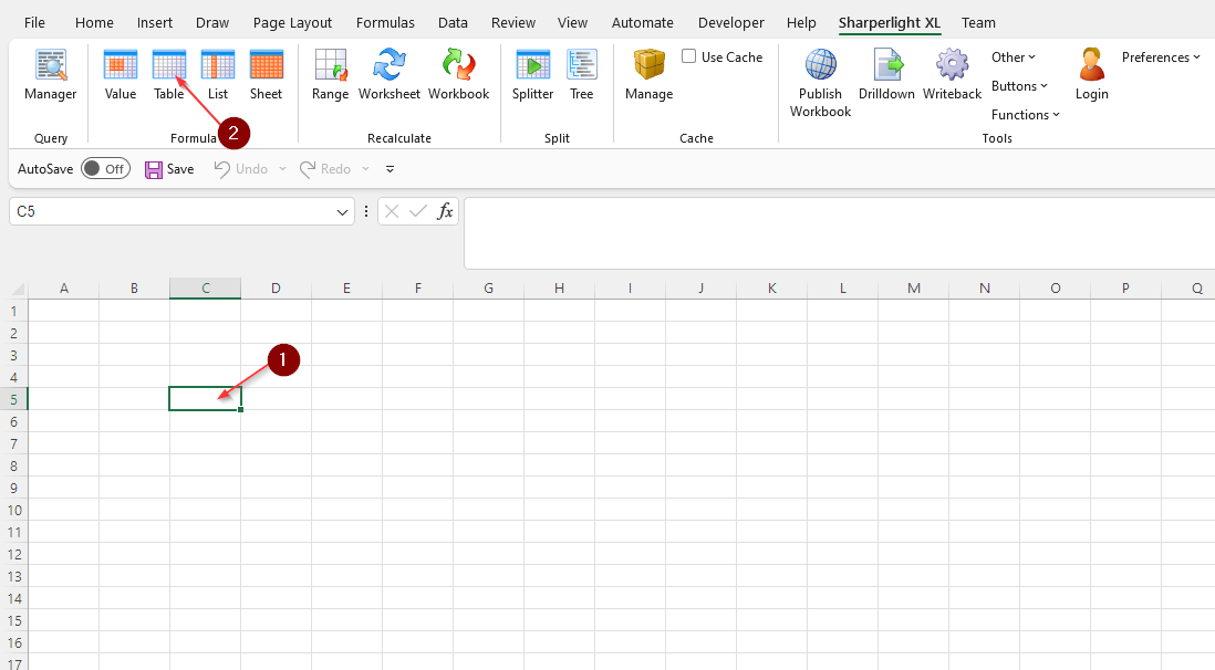
Open Excel and select 1. cell C5, then click on the 2. Table icon in the Sharperlight ribbon to launch the Query Builder.
Specifying Filters
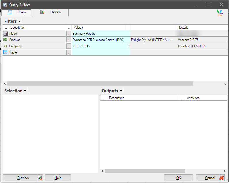
This corresponds to the FROM and WHERE clauses in SQL statements. In this case, we will use the Dynamics 365 Business Central as the data source, specifically focusing on the Product. Let's proceed with the Company set to <DEFAULT>.
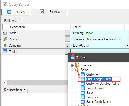
Specify Cust. Ledger Entry for the Table.
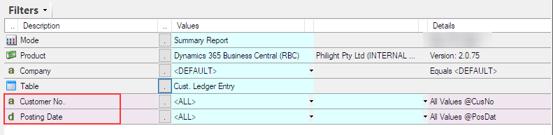
Upon selecting this table, two mandatory filters, namely Customer No. and Posting Date, will automatically appear. For both of these filters, we will keep the filter values as <ALL> for this instance.
On the lower-left side, a tree structure will display the selected table's columns and JOIN information.
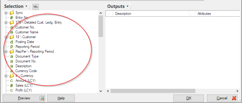
From here, you can select the columns you want to use for output and the columns you want to use as filters. Let's proceed by dragging and dropping the Document No., Due Date, and Open columns into the filter area.
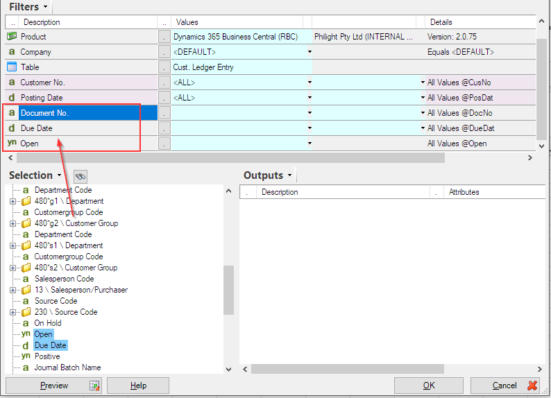
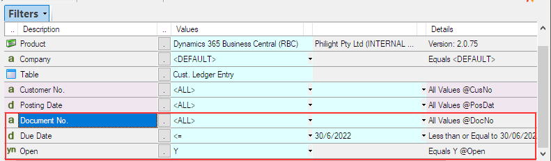
Here are the specified values for each:
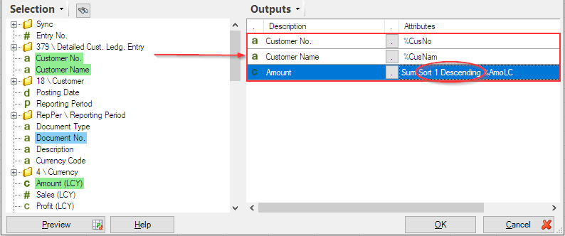
Specifying Output Items
This corresponds to the SELECT clause in SQL statements. Double-click or drag and drop the columns you want to display as query results from the selection tree view to the output area. For this instance, we will output these three columns. Additionally, the Amount column has been sorted in descending order.
Preview and Confirm
Let's validate the query by pressing the Preview button.
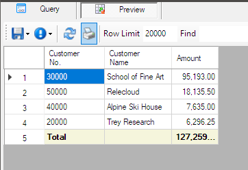
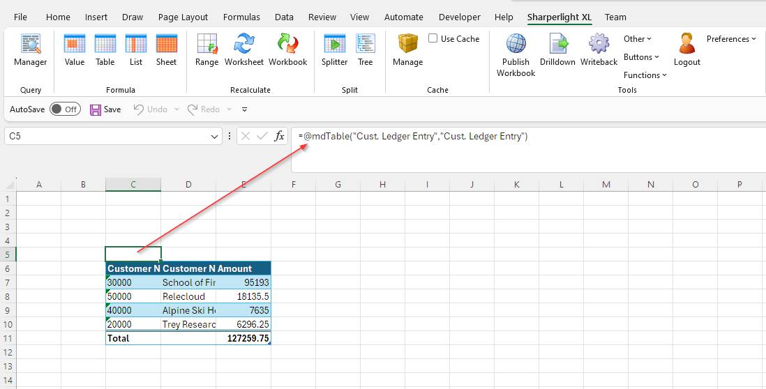
Everything worked correctly, so let's use the OK button to expand the data onto Excel. The Sharperlight table formula is defined in Cell C5, and a table has been created starting from the cell just below it.
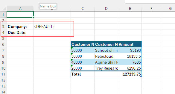
Improvement with Cell References for Filters
Let's make this report a bit more user-friendly. In Cell A3 and Cell A4, enter the following values. Also, in Cell B3, enter <DEFAULT>.
Double-click on Cell C5 to invoke the query definition.
First, 1. Select the value field for the Company filter in the query builder. Then, 2. double-click on Cell B3.
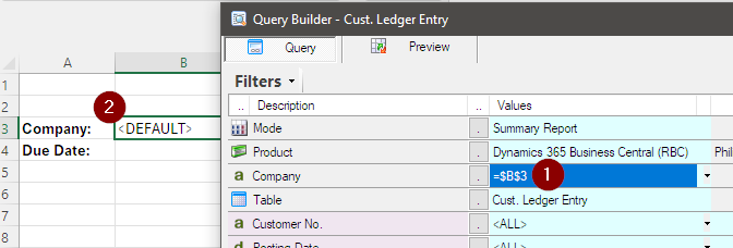
The formula referencing Cell B3 will be set as the value field for the Company filter in the query builder.
Similarly, 1. select the value field on the right side of the Due Date filter in the query builder. Then, 2. double-click on Cell B4.
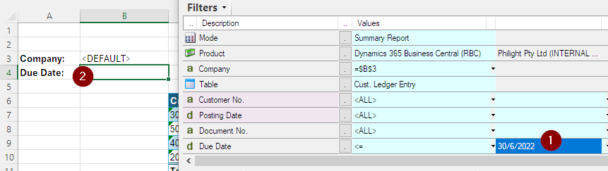
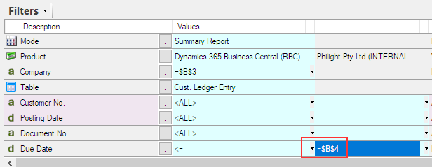
The formula referencing Cell B4 will be set as the value field for the right side of the Due Date filter in the query builder.
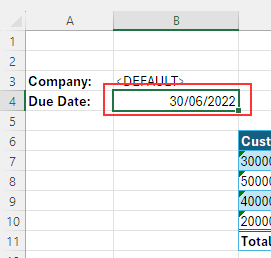
Set Cell B4 with the date value 30/06/2022.
The query modification is now complete. Reflect the changes by clicking the OK button in the query builder.
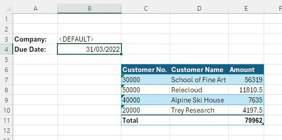
Now, the values entered in Cell B3 and Cell B4 will be reflected in the Sharperlight table formula (query) filters. Try double-clicking on Cell B4. This should open a date selection dialog.
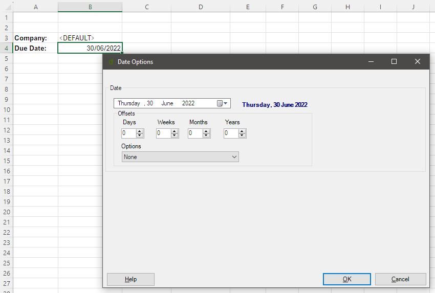
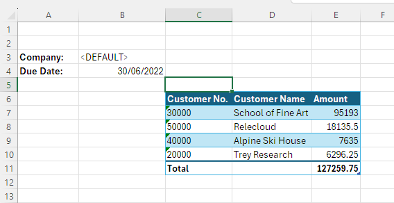
If you select a different date, the query will be recalculated immediately.
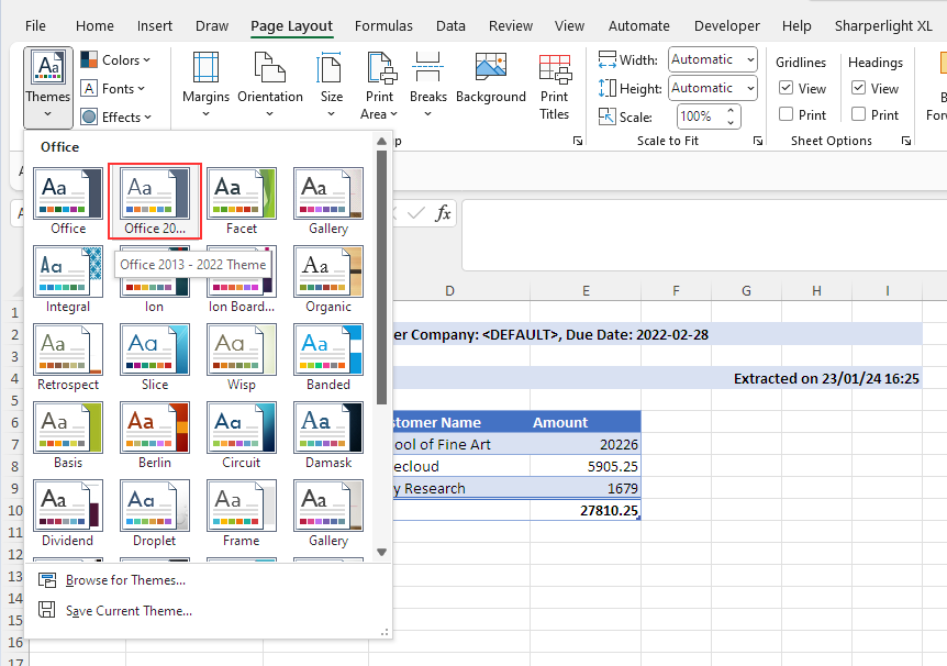
I will change the background color of filter cells and organize the report. I will use Excel's standard themes.
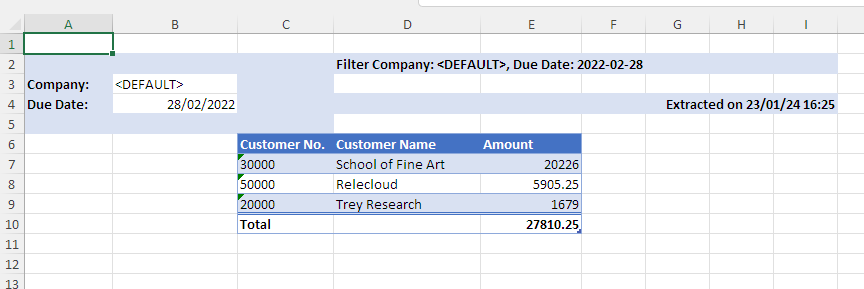
Conclusion
What do you think? It seems like creating a report is easy.