これまでの復習も兼ねて機械学習の流れを一通りやりたいと思います。
目次
扱うデータ
前処理
実行結果と手法の比較
ハイパーパラメータチューニング
扱うデータ
KaggleにあるTitanic号の生存者のデータ。
Titanic号に乗った人が生存するか否か予測するモデルを作ります。
前処理
いざ解析・・・の前にプログラムが処理しやすいよう形を整える必要があります。
データの確認と分割
まずはデータの確認をしましょう。
import numpy as np # linear algebra
import pandas as pd # data processing, CSV file I/O (e.g. pd.read_csv)

import os
for dirname, _, filenames in os.walk('/kaggle/input'):
    for filename in filenames:
        print(os.path.join(dirname, filename))

train = pd.read_csv('../input/titanic/train.csv')
test = pd.read_csv('../input/titanic/test.csv')
gender_submission = pd.read_csv('../input/titanic/gender_submission.csv')

train.head()#学習データの中身を見る
結果

読み込めました。
今回予測したいのはSurvivedの値です。このSurvived列とそれ以外に分けましょう。
X = train.drop('Survived',axis=1)
y = train.loc[:,"Survived"] # survivedを正解データ

X.head()

Xからsurvivedが消えました。
不要情報の削除と補間
ここでは不要なデータの削除と補間を行います。
不要情報の削除
予測に関係なさそうな値を削除していきます。
ここではName,Ticket(チケット番号),Cabin(客室番号)は不要だと判断しました(もちろん吟味する必要がありますが割愛)
# 特徴データになりえないものを削除
X = X.drop(['Name','Ticket','Cabin'],axis=1)
X.head()
欠損値の確認
まず欠損値がどこにあるか確認します。
# 欠損列の確認
X.isnull().any()
結果
PassengerId    False
Pclass         False
Sex            False
Age             True
SibSp          False
Parch          False
Fare           False
Embarked        True
dtype: bool
AgeとEmbarked(意味:どこから来たか)にあります。
欠損値に注意しながらデータの処理を進めます。
one-hot-encording
ここでは文字列を数値列に変換します。
例えば'Sex'列に'male'と'female'があるのでこちらを数値化0と1します。
# one_hot_encording
ohe_columns = ['Sex','Pclass','Embarked']

X_new = pd.get_dummies(X,
                       dummy_na=True,
                       columns=ohe_columns)#dummy_na=Trueとすれば欠損値の情報も抜き出せます。

X_new.head()
結果

Sex_female,Sex_male,Sex_nanという新しい列ができました。
連続値の欠損値処理
次にAgeの欠損値処理です。
連続値なのでOne-hot-encordingは使えません。
そこで平均値補間を使います。
from sklearn.impute import SimpleImputer

## 欠損値NaNを平均値で置換
imp = SimpleImputer()
imp.fit(X_new)

# X_newの欠損値を置換
X_ohe_columns = X_new.columns.values
X_ohe = pd.DataFrame(imp.transform(X_new), columns=X_ohe_columns)

X_ohe.isnull().any()
結果
Age             False
SibSp           False
Parch           False
Fare            False
Sex_female      False
Sex_male        False
Sex_nan         False
Pclass_1.0      False
Pclass_2.0      False
Pclass_3.0      False
Pclass_nan      False
Embarked_C      False
Embarked_Q      False
Embarked_S      False
Embarked_nan    False
dtype: bool
欠損値がなくなりました。
今回はここで前処理を終えますが、特徴量が多い場合特徴量抽出などを行って次元削減をします。
実行結果と手法の比較
ここでは手法の検討(ロジスティック分類がいいのか勾配ブースティングがいいのか等々)を行います。
import numpy as np
import pandas as pd
from sklearn.preprocessing import StandardScaler
from sklearn.neighbors import KNeighborsClassifier
from sklearn.linear_model import LogisticRegression
from sklearn.svm import SVC, LinearSVC
from sklearn.tree import DecisionTreeClassifier
from sklearn.ensemble import RandomForestClassifier
from sklearn.ensemble import GradientBoostingClassifier
from sklearn.neural_network import MLPClassifier
from sklearn.pipeline import Pipeline
from sklearn.model_selection import train_test_split
from sklearn.metrics import accuracy_score


# ホールドアウト

X_train, X_test,y_train,y_test=train_test_split(
    X_ohe, y, random_state=0
)


pipelines = {
    'knn':
        Pipeline([('scl',StandardScaler()),
                  ('est',KNeighborsClassifier())]),
    'logistic':
        Pipeline([('scl',StandardScaler()),
                  ('est',LogisticRegression(random_state=1))]),
    'rsvc':
        Pipeline([('scl',StandardScaler()),
                  ('est',SVC(C=1.0, kernel='rbf', class_weight='balanced', random_state=1))]),
    'lsvc':
        Pipeline([('scl',StandardScaler()),
                  ('est',LinearSVC(C=1.0, class_weight='balanced', random_state=1))]),
    'tree':
        Pipeline([('scl',StandardScaler()),
                  ('est',DecisionTreeClassifier(random_state=1))]),
    'rf':
        Pipeline([('scl',StandardScaler()),
                  ('est',RandomForestClassifier(random_state=1))]),
    'gb':
        Pipeline([('scl',StandardScaler()),
                  ('est',GradientBoostingClassifier(random_state=1))]),
    'mlp':
        Pipeline([('scl',StandardScaler()),
                  ('est',MLPClassifier(hidden_layer_sizes=(3,3),
                                       max_iter=1000,
                                       random_state=1))])
}

scores = {}
for pipe_name, pipeline in pipelines.items():
    pipeline.fit(X_ohe, y)
    scores[(pipe_name,'train')] = accuracy_score(y_train, pipeline.predict(X_train))
    scores[(pipe_name,'test')] = accuracy_score(y_test, pipeline.predict(X_test))

pd.Series(scores).unstack()
結果

ってなわけでテストデータに対する正答率が高いランダムフォレストか決定木がよさそうです。
ハイパーパラメータチューニング
最後にハイパーパラメータをチューニングします。
今回は一番スコアが良い決定木のmax_depthで行います
from sklearn import preprocessing
sscaler = preprocessing.StandardScaler()
X_s_train = sscaler.fit_transform(X_train) # xを正規化

param_grid_svm = {'max_depth':[1,2,3,4,5,6,7,8,9]}

from sklearn.model_selection import GridSearchCV
grid_search=GridSearchCV(DecisionTreeClassifier(random_state=1),param_grid_svm)
grid_search.fit(X_s_train, y_train)

print("Best parameters:{}".format(grid_search.best_params_))
print("Best cross-validation score:{}".format(grid_search.best_score_))
print("Best estimator:\n{}".format(grid_search.best_estimator_))
結果
Best parameters:{'max_depth': 3}
Best cross-validation score:0.8233980473571991
Best estimator:
DecisionTreeClassifier(ccp_alpha=0.0, class_weight=None, criterion='gini',
                       max_depth=3, max_features=None, max_leaf_nodes=None,
                       min_impurity_decrease=0.0, min_impurity_split=None,
                       min_samples_leaf=1, min_samples_split=2,
                       min_weight_fraction_leaf=0.0, presort='deprecated',
                       random_state=1, splitter='best')
max_depthは3がよさそうでした。
max_depthを変化させたときの様子を確認してみましょう。
import pandas as pd
import numpy as np
import matplotlib.pyplot as plt

results=pd.DataFrame(grid_search.cv_results_)

scores=np.array(results.mean_test_score)
plt.plot([1,2,3,4,5,6,7,8,9],scores)
plt.xlabel("max_depth")
plt.ylabel("test_score")
結果
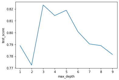
やはり3が最もテスト誤差が少なくなります。
今回はここまで。
参考文献
Pythonではじめる機械学習――scikit-learnで学ぶ特徴量エンジニアリングと機械学習の基礎