Intro
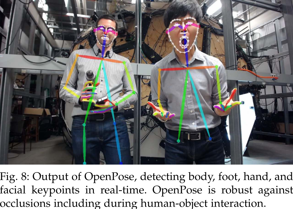
This article will digest OpenPose, a deep learning approach to solve human pose estimation problem:
-
Cao, Z., Simon, T., Wei, S. E., & Sheikh, Y. (2017). Realtime multi-person 2D pose estimation using part affinity fields. Proceedings - 30th IEEE Conference on Computer Vision and Pattern Recognition, CVPR 2017, 2017-Janua(Xxx), 1302–1310. https://doi.org/10.1109/CVPR.2017.143
-
Benchmark: Here
Clarification: OpenPose is the name of an evolving python library rather than the name of algorithm. In this blog, OpenPose specifically refers to the original OpenPose algorithm as cited above.
The Pose Challenge
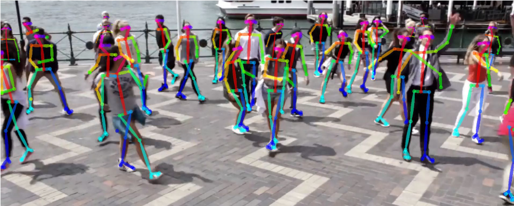
The challenge is pretty straight. Given a picture of multiple people, AI is asked to annotate the position of limb of each person in the picture: such as left hand, right arm, nose and many others. Note: in this paper, limb is the pair of annotated positions of human, a more general definition.

Difficulties
There are mainly two ways to solve this challenge: Top-down and Bottom-up.
Traditional top-down strategy finds out the part of each person firstly, then analyzes each person to find out limbs. It does not work well because:
Humans are hard to find. If you failed this step, the whole process would mess up. To precisely find out each part of people especially when they overlap each other, we need methods from another area, Semantic Segmentation, which is makes the problem too complex.
Top-down fails to use global information which is very useful when people are too close to each other (and they are likely to).
On the other hand, traditional bottom-up method tends to give part proposals firstly (hands, legs, etc.,), then to assign them to each person. It does not work well either because:
Sometimes the proposed algorithms are NP-hard.
Even after improved with better methods, it takes too much time to compute with many unwanted limitations.
OpenPose Overview
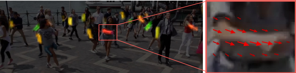
OpenPose takes a bottom-up style with two steps. First, instead of looking for parts directly, it looks for a Part Affinity Field (PAF) for each pixel that indicates the direction of (possible) limb at this place. Second, OpenPose uses the original picture information along with predicted PAFs to generate a confidence map, which is the candidate points of limb joint.
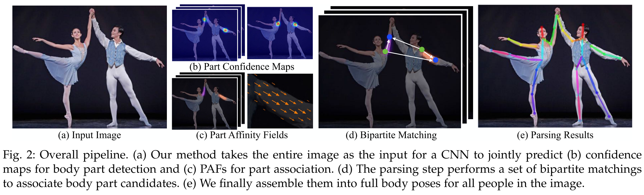
Look at the figure below for a general idea about PAF and the whole procedure.
Step 1: PAF Prediction
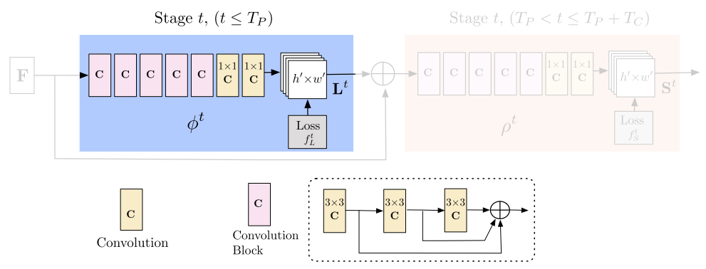
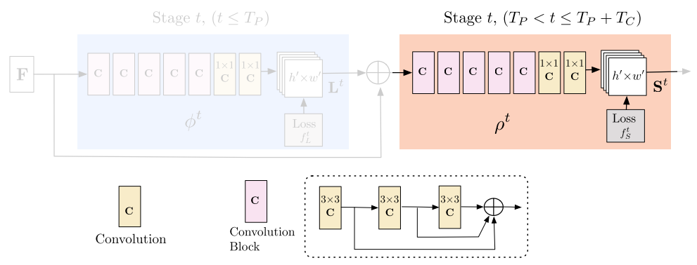
Note, the blue part will loop for many times which is called stages in the paper. In each subsequent stage, the predictions from the previous stage and the original image features $\mathrm{F}$ are concatenated. Then they are used to compute PAF predictions, $ \mathrm{L}^t = \phi^t(\mathrm{F},\mathrm{L}^{t-1}), t = 2 \dots T_P \tag{1} $$ $where $\phi^t$ refers to the CNNs in the blue part of the figure and $T_P$ refers to the number of PAF stages.
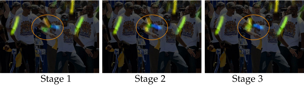
This figure shows how stages loop increase the quality of estimates. It is mostly due to empirical optimization instead of theoretical ones. (So the paper does not know mathematically why.)
Loss function is applied at the end of EACH stage as following:
$$f^{t_i}_\mathrm{L} = \sum_{c=1}^C \sum_\mathrm{p} \mathrm{W}(\mathrm{p}) \cdot || \mathrm{L}^{t_i}_c(\mathrm{p}) - \mathrm{L}^*_c(\mathrm{p}) ||^2_2 \tag{2}$$
where $\mathrm{L}_c^*$ is the groundtruth PAF. $\mathrm{W}(\mathrm{p}) \doteq 0$ if there is no annotated groundtruth at the pixel $\mathrm{p}$.
Groundtruth will be explained later.
Step 2: Confidence Map Prediction
Similar to the PAF part, Confidence Map Prediction will loop for $T_C$ stages. Its initial input is the final result from the PAF part, along with the original information concatenated. Then it performs similar computations as in the PAF part:
Loss function is also defined similarly:
$$ f^{t_i}_\mathrm{S} = \sum_{j=1}^J \sum_\mathrm{p} \mathrm{W}(\mathrm{p}) \cdot || \mathrm{S}^{t_k}_c(\mathrm{p}) - \mathrm{S}^*_c(\mathrm{p}) ||^2_2 \tag{3} $$
Groundtruth for PAF
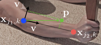
For each point predicted by the PAF part, its groundtruth PAF must be computed. The annotated labels we have are positions of limb joint like $x_{j_1,k}$ in the figure above. The paper deploys a straight forward solution:
Each pixel $\mathrm{p}$ is compared with all joint in the picture to generate vectors. Groundtruth should equal to their sum.
For a single person's single joint, the groundtruth should be the true unit vector that points to the right direction, or, $\mathrm{v}$ in the figure above.
Pixels that are too far away or in the wrong direction should receive zero vector for this joint.
If the pixel $\mathrm{p}$ is NOT on the limb, it should receive zero vector. We can measure it by comparing $|\mathrm{v}_\perp \cdot \mathrm{p} - x_{j_1,k}|$ with a threshold $\sigma_l$
Mathematically: $$ \mathrm{L}_{c,k}^*(\mathrm{p}) = \begin{cases} \mathrm{v}\quad \text{ if } \mathrm{v} \text{ on limb } c,k \ 0 \quad \text{ otherwise }. \end{cases} $$
Then, the groundtruth PAF averages individual ones as:
$$ \mathrm{L}^_c(\mathrm{p}) = \frac{1}{n_c(\mathrm{p})}\sum_k \mathrm{L}^_{c,k}(\mathrm{p}) $$
where $n_c(\mathrm{p})$ is the number of non-zero vectors at point $\mathrm{p}$ across all $k$ people.
During testing, paper measures the association between candidate part detections by computing the line integral over the corresponding PAF along the line connecting the candidate part. Specifically, for two candidate part locations $d_{j_1}$ and $d_{j_2}$, paper samples the predicted PAF, $\mathrm{L}_c$ to measure the confidence:
$$ E = \int_{u=0}^{u=1} \mathrm{L}_c(\mathrm{p}(u))\cdot \frac{\mathrm{d}_{j_2} - \mathrm{d}_{j_1}}{ || \mathrm{d}_{j_2} - \mathrm{d}_{j_1} ||_2 } du $$
where $\mathrm{p}(u)$ interpolates the position of the two body parts $d_{j_1}$ and $d_{j_2}$. Well in practice, for the sake of efficiency, we approximate it by sampling and summing uniformly-spaced values of $u$.
Groundtruth for Confidence Maps
Each confidence map is a 2D representation of the belief that a particular body part can be located in any given pixel. Ideally, if a single person appears in the image, a single peak corresponding to the part of the limb should appear. The groundtruth is generated as a gaussian distribution from the annotated points:
Let $\mathrm{x}_{j,k} \in \mathbb{R}^2$ be the groundtruth position of body part $j$ for person $k$ in the image. Then, the value at location $\mathrm{p} \in \mathbb{R}^2$ in $\mathrm{S}_{j,k}^*$ is defined as,
$$ \mathrm{S}^*_{j,k}(\mathrm{p}) = \exp \big( - \frac{ || \mathrm{p} - \mathrm{x}_{j,k} ||^2_2 }{\sigma^2} \big) $$
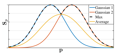
where $\sigma$ controls the spread of the peak. It is for a particular person $k$, and the global one would be the max of those individual values:
$$ \mathrm{S}_j^(\mathrm{p}) = \max_k \mathrm{S}^_{j,k}(\mathrm{p}). $$
The reason paper uses maximum rather than average is to remain peaks distinct. At test time, paper uses non-maximum suppression to filter candidates.
Multi-Person Parsing
After performing non-maximum suppression on the detection confidence maps to obtain the set of candidate points, we have to assign these points to limbs.
We can use line integral $E$ to describe 'score' of each possible limb. Given two points that are proposed by the confidence map, we only pick the CONNECTED ones that have HIGHEST $E$. We perform such greedy actions to all points in the graph like the following:
In order to solve the complexity problem, paper uses Bipartite Graphs relaxations on a spanning tree skeleton of human poses to reduce the optimization to:
$$ \max_Z E = \sum_{c=1}^C \max_{Z_c} E_c $$
Conclusion
OpenPose uses the PAF and several optimizations to produce stable and relatively fast result. (Faster in this improvement).
In this article, I introduce the basic algorithm and intuition. For further info, please refer to the original paper. It is quite readable. :)
Thank you for reading. Cheers!