はじめに
多変数の回帰モデルをやろうとしており、数ある機械学習の手法をいくつかピックアップして、精度を比較検証したい。
scikit-learnというPythonの機械学習ライブラリには、色々と実装されており便利なので、サクッと使ってやってみた。
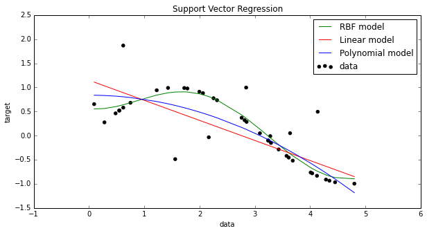
まずデモ
Examplesで紹介されているのが以下、
import numpy as np
from sklearn.svm import SVR
import matplotlib.pyplot as plt
%matplotlib inline

# インプットを乱数で生成
X = np.sort(5 * np.random.rand(40, 1), axis=0)
# アウトプットはsin関数
y = np.sin(X).ravel()

# アウトプットにノイズを与える
y[::5] += 3 * (0.5 - np.random.rand(8))

# RBFカーネル、線形、多項式でフィッティング
svr_rbf = SVR(kernel='rbf', C=1e3, gamma=0.1)
svr_lin = SVR(kernel='linear', C=1e3)
svr_poly = SVR(kernel='poly', C=1e3, degree=2)
y_rbf = svr_rbf.fit(X, y).predict(X)
y_lin = svr_lin.fit(X, y).predict(X)
y_poly = svr_poly.fit(X, y).predict(X)

# 図を作成
plt.figure(figsize=[10, 5])
plt.scatter(X, y, c='k', label='data')
plt.hold('on')
plt.plot(X, y_rbf, c='g', label='RBF model')
plt.plot(X, y_lin, c='r', label='Linear model')
plt.plot(X, y_poly, c='b', label='Polynomial model')
plt.xlabel('data')
plt.ylabel('target')
plt.title('Support Vector Regression')
plt.legend()
plt.show()
結果:
実際にやってみた
条件
- 4変数(4次元)
- 学習データセットとテストデータセットを用意
- 学習させた後、テストデータをつっこんで推定
- RBF、線形、多項式の推定精度を比較
- 推定精度は、RMSEと相関係数を使う
import numpy as np
from sklearn.svm import SVR
import matplotlib.pyplot as plt

# インプットを適当に生成
X1 = np.sort(5 * np.random.rand(40, 1).reshape(40), axis=0)
X2 = np.sort(3 * np.random.rand(40, 1).reshape(40), axis=0)
X3 = np.sort(9 * np.random.rand(40, 1).reshape(40), axis=0)
X4 = np.sort(4 * np.random.rand(40, 1).reshape(40), axis=0)

# インプットの配列を一つに統合
X = np.c_[X1, X2, X3, X4]

# アウトプットを算出
y = np.sin(X1).ravel() + np.cos(X2).ravel() + np.sin(X3).ravel() - np.cos(X4).ravel()

y_o = y.copy()

# ノイズを加える
y[::5] += 3 * (0.5 - np.random.rand(8))

# フィッティング
svr_rbf = SVR(kernel='rbf', C=1e3, gamma=0.1)
svr_lin = SVR(kernel='linear', C=1e3)
svr_poly = SVR(kernel='poly', C=1e3, degree=3)
y_rbf = svr_rbf.fit(X, y).predict(X)
y_lin = svr_lin.fit(X, y).predict(X)
y_poly = svr_poly.fit(X, y).predict(X)

# テストデータも準備
test_X1 = np.sort(5 * np.random.rand(40, 1).reshape(40), axis=0)
test_X2 = np.sort(3 * np.random.rand(40, 1).reshape(40), axis=0)
test_X3 = np.sort(9 * np.random.rand(40, 1).reshape(40), axis=0)
test_X4 = np.sort(4 * np.random.rand(40, 1).reshape(40), axis=0)

test_X = np.c_[test_X1, test_X2, test_X3, test_X4]
test_y = np.sin(test_X1).ravel() + np.cos(test_X2).ravel() + np.sin(test_X3).ravel() - np.cos(test_X4).ravel()

# テストデータを突っ込んで推定してみる
test_rbf = svr_rbf.predict(test_X)
test_lin = svr_lin.predict(test_X)
test_poly = svr_poly.predict(test_X)
以下、検証
from sklearn.metrics import mean_squared_error
from math import sqrt

# 相関係数計算
rbf_corr = np.corrcoef(test_y, test_rbf)[0, 1]
lin_corr = np.corrcoef(test_y, test_lin)[0, 1]
poly_corr = np.corrcoef(test_y, test_poly)[0, 1]

# RMSEを計算
rbf_rmse = sqrt(mean_squared_error(test_y, test_rbf))
lin_rmse = sqrt(mean_squared_error(test_y, test_lin))
poly_rmse = sqrt(mean_squared_error(test_y, test_poly))

print "RBF: RMSE %f \t\t Corr %f" % (rbf_rmse, rbf_corr)
print "Linear: RMSE %f \t Corr %f" % (lin_rmse, lin_corr)
print "Poly: RMSE %f \t\t Corr %f" % (poly_rmse, poly_corr)
こんな結果になった
RBF: RMSE 0.707305 		 Corr 0.748894
Linear: RMSE 0.826913 	 Corr 0.389720
Poly: RMSE 2.913726 	 Corr -0.614328