ggplot2とfor構文を組み合わせて、一気に複数枚の作図をする
階層群集モデルの結果をCSVファイルに出力後、種ごとの結果を作図する際に使用したコードです。
前半は気合が入ってますが、後半に行くにつれてとてもコードが汚くなっています...
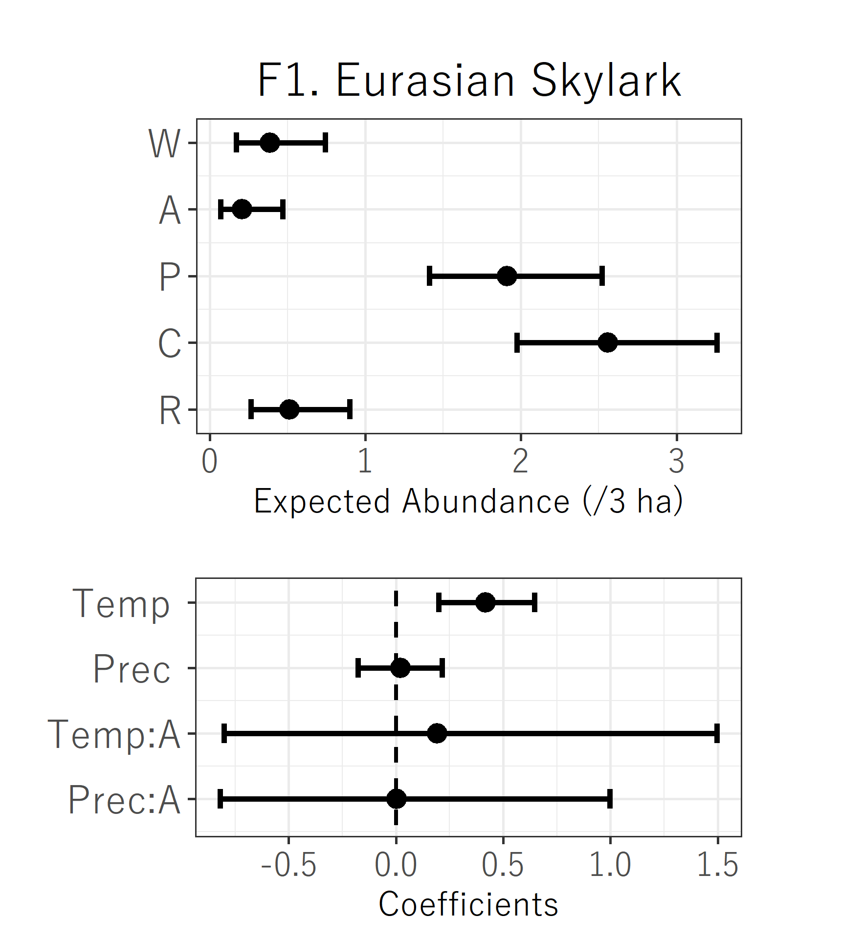
最終的には、こんな画像が種ごとに描けます。
library("ggplot2")                    ##ggplot2パッケージの読み込み
windowsFonts("YuGo" = windowsFont("游ゴシック"))    ##フォントの読み込み
library(gridExtra)
library(onemap)
library(png)
library(grid)

setwd("c:/Users/...") ##ディレクトリの指定
comm3 <- read.csv("結果ファイル.csv", header = F)                 ##MCMCの結果が入ったcsvファイル
comm4 <- read.csv("タイトルファイル.csv", header = F, stringsAsFactors=F)        ##一枚一枚の作図のタイトルを入力したcsvファイル

# 新たな297行3列のマトリックスを作成
# MCMCの結果が3種のハイパーパラメータと33種のパラメーター9個で、297行あるため
# MCMCの出力結果から描写に使うのが、中央値・95%信用区間の上端と下端なので3列分
x <- matrix(NA,297,3)

x[,1] <- comm3[,4] # comm3の結果のうちの4列目のみ抜き出してxに付加
x[,2] <- comm3[,5] # comm3の結果のうちの5列目のみ抜き出してxに付加
x[,3] <- comm3[,6] # comm3の結果のうちの6列目のみ抜き出してxに付加

# 新たな21行1列のマトリックスを作成
p <- matrix(NA,297,1)

p[,1] <- comm4[,1]
# 別途作成していたタイトルファイルについても行列を作成、ここでは種名(F1. Eurasian Skylark)に該当する文が33種ぶん含まれている


####################################################################
################## plotting each species#############################
####################################################################
value <-  0:32
for (z in 0:32){

res <- paste("plot",z, sep="")
    eval(call("<-", as.name(z),value))
sum <- data.frame(sx = c(5,4,3,2,1),
                  sy = c(exp(x[9*z+1,1]),exp(x[9*z+2,1]),
                       exp(x[9*z+3,1]),exp(x[9*z+4,1]),exp(x[9*z+5,1])))
#### データを指定する数列を作成、ここではパラメータW, A, P, C, Rの部分を指定


sum2 <- data.frame(sx = c(1,2,3,4),
                   sy = c(x[9*z+9,1],x[9*z+8,1],x[9*z+7,1],x[9*z+6,1]))
#### データを指定する数列を作成、ここではパラメータTemp, Prec, Temp:A, Prec:Aの部分を指定

#### 以下、コード汚い
c1 <-exp(x[9*z+1,2])                                             ####Lower 95% CI of W
c2 <-exp(x[9*z+2,2])                                             ####Lower 95% CI of A
c3 <-exp(x[9*z+3,2])                                             ####Lower 95% CI of P
c4 <-exp(x[9*z+4,2])                                             ####Lower 95% CI of C
c5 <-exp(x[9*z+5,2])                                             ####Lower 95% CI of R
c6 <-exp(x[9*z+1,3])                                             ####Upper 95% CI of W
c7 <-exp(x[9*z+2,3])                                             ####Upper 95% CI of A
c8 <-exp(x[9*z+3,3])                                             ####Upper 95% CI of P
c9 <-exp(x[9*z+4,3])                                             ####Upper 95% CI of C
c10<-exp(x[9*z+5,3])                                             ####Upper 95% CI of R

tem1 <-x[9*z+6,2]                                                ####Lower 95% CI of Temp
tem2 <-x[9*z+6,3]                                                ####Upper 95% CI of Temp
pre1 <-x[9*z+7,2]                                                ####Lower 95% CI of Prec
pre2 <-x[9*z+7,3]                                                ####Upper 95% CI of Prec
tema1 <-x[9*z+8,2]                                               ####Lower 95% CI of Temp
tema2 <-x[9*z+8,3]                                               ####Upper 95% CI of Temp
prea1 <-x[9*z+9,2]                                               ####Lower 95% CI of Prec
prea2 <-x[9*z+9,3]                                               ####Upper 95% CI of Prec
name  <-p[9*z+1,1]                                               ####name


#### ここから作図、まず上半分
lnduse <- ggplot(comm3) +
       theme_bw(base_size=11, base_family='') +
       xlim(0,5) +
       scale_x_reverse() +
       scale_x_continuous(breaks=c(1,2,3,4,5),
                          labels=c("R","C","P","A","W"))+
       xlab("") + ylab("Abundance (/3 ha)")+
       geom_errorbar(mapping = aes(x = 1, ymin=c5, ymax =c10),
                        size = 1, width = 0.3, color = "black") +
       geom_errorbar(mapping = aes(x = 2, ymin=c4 , ymax =c9),
                        size = 1, width = 0.3, color = "black") +
       geom_errorbar(mapping = aes(x = 3, ymin=c3 , ymax =c8),
                        size = 1, width = 0.3, color = "black") +
       geom_errorbar(mapping = aes(x = 4, ymin=c2 , ymax =c7),
                        size = 1, width = 0.3, color = "black") +
       geom_errorbar(mapping = aes(x = 5, ymin=c1 , ymax =c6),
                        size = 1, width = 0.3, color = "black") +
       geom_point(data = sum, aes(x = sx, y = sy),
                  size = 3, color = "black") +
       labs(title = name) +
       theme(plot.title = element_text(hjust = 0.5),
             text = element_text(size = 12, family = "YuGo"))+
       theme(axis.title.x = element_text(size=12, family = "YuGo"),
             axis.title.y = element_text(size=8, family = "YuGo")) +
       theme(axis.text.x = element_text(size=12, family = "YuGo"),
             axis.text.y = element_text(size=14, family = "YuGo")) +
       guides(fill = FALSE) +
       coord_flip()


#### ここ以下も作図、下半分に相当
coeff  <- ggplot(comm3) +
       theme_bw(base_size=11, base_family='') +
       xlim(0,4.2) +
       scale_x_reverse() +
       scale_x_continuous(breaks=c(1,2,3,4),
                          labels=c("Prec:A", "Temp:A","Prec ","Temp "))+
       xlab("") + ylab("Coefficients")+
       geom_errorbar(mapping = aes(x = 1, ymin=prea1, ymax =prea2),
                        size = 1, width = 0.3, color = "black") +
       geom_errorbar(mapping = aes(x = 2, ymin=tema1, ymax =tema2),
                        size = 1, width = 0.3, color = "black") +
       geom_errorbar(mapping = aes(x = 3, ymin=pre1, ymax =pre2),
                        size = 1, width = 0.3, color = "black") +
       geom_errorbar(mapping = aes(x = 4, ymin=tem1, ymax =tem2),
                        size = 1, width = 0.3, color = "black") +
       geom_segment(aes(x=0.6, y=0, xend=4.2, yend=0), linetype = 2,size=0.7, color = "black") +
       geom_point(data = sum2, aes(x = sx, y = sy),
                  size = 3, color = "black") +
       theme(plot.title = element_text(hjust = 0.5),
             text = element_text(size = 14, family = "YuGo"))+
       theme(axis.title.x = element_text(size=12, family = "YuGo"),
             axis.title.y = element_text(size=8, family = "YuGo")) +
       theme(axis.text.x = element_text(size=12, family = "YuGo"),
             axis.text.y = element_text(size=14, family = "YuGo")) +
       guides(fill = FALSE) +
       coord_flip()

res <- ggdraw() +
          draw_plot(lnduse, x = 0.12, y = 0.43, width = 0.78, height = 0.52) +
          draw_plot(coeff,  x = 0, y = 0, width = 0.9, height = 0.40)
res
ggsave(plot = res, file = paste("RES190526/INtSpecies", z, ".png", sep=""),
       width = 4.3, height = 4.8, dpi = 400)}