(base) $ conda create -n py37_manifold python=3.7 anaconda
(base) $ source activate py37_manifold
(py37_manifold) $
autograd インストール
(py37_manifold) $ pip install autograd

Collecting autograd
  Downloading autograd-1.3.tar.gz (38 kB)
Requirement already satisfied: numpy>=1.12 in ./.pyenv/versions/anaconda3-5.2.0/envs/py37_manifold/lib/python3.7/site-packages (from autograd) (1.20.1)
Requirement already satisfied: future>=0.15.2 in ./.pyenv/versions/anaconda3-5.2.0/envs/py37_manifold/lib/python3.7/site-packages (from autograd) (0.18.2)
Building wheels for collected packages: autograd
  Building wheel for autograd (setup.py) ... done
  Created wheel for autograd: filename=autograd-1.3-py3-none-any.whl size=47989 sha256=5c0ad6c3fbd42a402118ce0201e9446001f6b34f6f61d4b1d34905856546eab6
  Stored in directory: /home/[user_name]/.cache/pip/wheels/ef/32/31/0e87227cd0ca1d99ad51fbe4b54c6fa02afccf7e483d045e04
Successfully built autograd
Installing collected packages: autograd
Successfully installed autograd-1.3
pip install pymanopt
pip install pymanopt

Collecting pymanopt
  Downloading pymanopt-0.2.5-py3-none-any.whl (59 kB)
     |████████████████████████████████| 59 kB 8.3 MB/s
Requirement already satisfied: numpy>=1.16 in ./.pyenv/versions/anaconda3-5.2.0/envs/py37_manifold/lib/python3.7/site-packages (from pymanopt) (1.20.1)
Requirement already satisfied: scipy in ./.pyenv/versions/anaconda3-5.2.0/envs/py37_manifold/lib/python3.7/site-packages (from pymanopt) (1.6.2)
Installing collected packages: pymanopt
Successfully installed pymanopt-0.2.5
simple example
import autograd.numpy as np

from pymanopt.manifolds import Stiefel
from pymanopt import Problem
from pymanopt.solvers import SteepestDescent

# (1) Instantiate a manifold
manifold = Stiefel(5, 2)

# (2) Define the cost function (here using autograd.numpy)
def cost(X): return np.sum(X)

problem = Problem(manifold=manifold, cost=cost)

# (3) Instantiate a Pymanopt solver
solver = SteepestDescent()

# let Pymanopt do the rest
Xopt = solver.solve(problem)
print(Xopt)

##### result ####
Compiling cost function...
Computing gradient of cost function...
 iter		   cost val	    grad. norm
    1	-1.4015650825981624e-01	3.11267080e+00
    2	-2.3990107640612464e+00	2.04513436e+00
    3	-2.6112734104347544e+00	1.57854640e+00
    4	-3.0634139985391604e+00	5.57823862e-01
    5	-3.1596369194162239e+00	1.15449706e-01
    6	-3.1619163364504663e+00	4.52108520e-02
    7	-3.1621110359538047e+00	3.24263239e-02
    8	-3.1622727108364495e+00	5.56752756e-03
    9	-3.1622776332134630e+00	3.15987307e-04
   10	-3.1622776495823297e+00	2.52182846e-04
   11	-3.1622776563767903e+00	1.54478928e-04
   12	-3.1622776577606118e+00	1.23397289e-04
   13	-3.1622776601144684e+00	1.84594057e-05
   14	-3.1622776601611871e+00	6.74250561e-06
   15	-3.1622776601655738e+00	4.21226109e-06
   16	-3.1622776601674873e+00	2.37418501e-06
   17	-3.1622776601683746e+00	1.74615286e-07
Terminated - min grad norm reached after 17 iterations, 0.01 seconds.

[[-0.9231764   0.29072086]
 [-0.11354918 -0.51890635]
 [-0.20623625 -0.42621928]
 [-0.30163413 -0.33082138]
 [-0.03654288 -0.59591268]]
動くことを確認。
PCA (1番重要な成分)
{\bf Data} =
\begin{bmatrix}
x \\
y \\
z \\
\end{bmatrix}
\sim

\exp
\left[
- \frac{1}{2} ({\bf Data} - {\bf \mu})^T \Sigma^{-1} ({\bf Data} - {\bf \mu})
\right]
のような場合を考える。
[x,y,z] のデータが5000点あった場合に、このデータを主成分分析する。
結果としてcovariant matrix の固有ベクトルが出てくればOK
import numpy
import autograd.numpy as np

from pymanopt.manifolds import Stiefel
from pymanopt import Problem
from pymanopt.solvers import SteepestDescent

from matplotlib import pyplot
Generate data
mean = [0, 0, 0]
cov = [[4, 0, 0],
       [0, 100, 0],
       [0, 0, 1]]

x, y, z = np.random.multivariate_normal(mean, cov, 5000).T
Find primary component
# (1) Instantiate a manifold
manifold = Stiefel(3,1)

# (2) Define the cost function (here using autograd.numpy)
def cost(X):
    A = np.dot(np.dot(np.dot(np.transpose(X),Data), Data.T), X)

    return A #np.sum(X)

problem = Problem(manifold=manifold, cost=cost)

# (3) Instantiate a Pymanopt solver
solver = SteepestDescent()

# let Pymanopt do the rest
Xopt = solver.solve(problem)
print(Xopt)

### result ###
Compiling cost function...
Computing gradient of cost function...
 iter		   cost val	    grad. norm
    1	+5.2481256509930645e+03	3.05029353e+03
    2	+5.2438277680737319e+03	1.11796033e+04
    3	+5.2277299499084174e+03	9.76012298e+03
    4	+5.1832913753482308e+03	3.89396089e+03
    5	+5.1730543591517953e+03	2.25383446e+03
    6	+5.1674731117783276e+03	4.15006278e+03
    7	+5.1569814507044375e+03	1.77263618e+03
    8	+5.1548307584959221e+03	4.98835962e+03
    9	+5.1475628151428082e+03	3.46102793e+03
...
  160	+5.1177163774291039e+03	4.20826319e-03
  161	+5.1177163774290912e+03	4.00752296e-03
  162	+5.1177163774290766e+03	2.64975638e-03
  163	+5.1177163774290730e+03	5.44183447e-03
  164	+5.1177163774290630e+03	3.23481435e-03
  165	+5.1177163774290530e+03	2.77523335e-03
  166	+5.1177163774290530e+03	3.64588563e-03
Terminated - min stepsize reached after 166 iterations, 0.13 seconds.

[[ 2.86165457e-02]
 [-7.81434337e-04]
 [-9.99590157e-01]]
print('1st component')
print(Xopt[:,0])

###
1st component
[ 2.86165457e-02 -7.81434337e-04 -9.99590157e-01]
PCA (2番目に重要な成分まで)
# (1) Instantiate a manifold
manifold = Stiefel(3,2) #(3,M) 3-dimensional data, upto M components
# (2) Define the cost function (here using autograd.numpy)
def cost(X):
u1 = X[:,0]
u2 = X[:,1]
A = np.dot(np.dot(np.dot(np.transpose(u1),Data), Data.T), u1)
B = np.dot(np.dot(np.dot(np.transpose(u2),Data), Data.T), u2)
total = 10*A + B
return total
problem = Problem(manifold=manifold, cost=cost)
# (3) Instantiate a Pymanopt solver
solver = SteepestDescent()
# let Pymanopt do the rest
Xopt = solver.solve(problem)
print(Xopt)
### result ###
Compiling cost function...
Computing gradient of cost function...
iter cost val grad. norm
1 +4.5909422299787309e+05 6.73632726e+05
2 +3.9998838651279337e+05 8.60920616e+05
3 +3.7217143449324067e+05 1.09219324e+06
4 +2.9760867757966439e+05 4.61126532e+05
5 +2.6485839779132232e+05 5.88725860e+05
6 +2.4115454199115711e+05 4.13853795e+05
7 +2.3286327975641249e+05 5.18976670e+05
8 +2.1573780797139945e+05 1.82309867e+05
9 +2.0890522151030271e+05 4.42702316e+05
...
378 +7.1325205578285662e+04 2.28983102e-02
379 +7.1325205578285648e+04 4.54266215e-02
380 +7.1325205578285590e+04 3.48791035e-02
381 +7.1325205578285531e+04 2.98695457e-02
382 +7.1325205578285502e+04 1.62483957e-02
383 +7.1325205578285430e+04 2.44885487e-02
384 +7.1325205578285386e+04 2.96063775e-02
385 +7.1325205578285328e+04 2.70866242e-02
386 +7.1325205578285269e+04 1.77460039e-02
387 +7.1325205578285269e+04 3.29106454e-02
Terminated - min stepsize reached after 387 iterations, 0.46 seconds.
[[-2.86166598e-02 9.99582533e-01]
[ 7.81441481e-04 -3.96006759e-03]
[ 9.99590154e-01 2.86195374e-02]]
print('1st component')
print(Xopt[:,0])

print('2nd component')
print(Xopt[:,1])

###

1st component
[-2.86166598e-02  7.81441481e-04  9.99590154e-01]
2nd component
[ 0.99958253 -0.00396007  0.02861954]
PCA (3番目に重要な成分まで)
# (1) Instantiate a manifold
manifold = Stiefel(3,3) #(3,M) 3-dimensional data, upto M components

# (2) Define the cost function (here using autograd.numpy)
def cost(X):
    u1 = X[:,0]
    u2 = X[:,1]
    u3 = X[:,2]
    A = np.dot(np.dot(np.dot(np.transpose(u1),Data), Data.T), u1)
    B = np.dot(np.dot(np.dot(np.transpose(u2),Data), Data.T), u2)
    C = np.dot(np.dot(np.dot(np.transpose(u3),Data), Data.T), u3)

    total = 100*A + 10*B + C
    return total

problem = Problem(manifold=manifold, cost=cost)

# (3) Instantiate a Pymanopt solver
solver = SteepestDescent()

# let Pymanopt do the rest
Xopt = solver.solve(problem)
print(Xopt)


### result ###
Compiling cost function...
Computing gradient of cost function...
 iter		   cost val	    grad. norm
    1	+7.5515693235367984e+06	1.84313213e+07
    2	+7.5140587271768823e+06	1.82693517e+07
    3	+7.3652525450036600e+06	1.79735368e+07
    4	+6.7905087199882809e+06	1.67585726e+07
    5	+4.8652095463687042e+06	1.14282554e+07
    6	+3.3966843449406191e+06	3.87973088e+06
    7	+3.1966327865994191e+06	4.20827848e+06
    8	+3.0344506122366516e+06	4.16634281e+06
    9	+2.8484096269338191e+06	3.03847060e+06
...
  202	+1.1948746632160679e+06	2.20285927e-01
  203	+1.1948746632160579e+06	4.73657545e-01
  204	+1.1948746632160575e+06	5.18645036e-01
  205	+1.1948746632160563e+06	3.58986049e-01
  206	+1.1948746632160549e+06	2.63097893e-01
  207	+1.1948746632160544e+06	2.39725167e-01
  208	+1.1948746632160537e+06	1.50571670e-01
  209	+1.1948746632160535e+06	1.06912027e-01
  210	+1.1948746632160530e+06	1.69717464e-01
  211	+1.1948746632160530e+06	3.12776693e-01
Terminated - min stepsize reached after 211 iterations, 0.33 seconds.

[[ 2.86165557e-02 -9.99582536e-01  3.98080911e-03]
 [-7.81442415e-04  3.96006767e-03  9.99991854e-01]
 [-9.99590157e-01 -2.86194333e-02 -6.67792694e-04]]
print('1st component')
print(Xopt[:,0])

print('2nd component')
print(Xopt[:,1])

print('3rd component')
print(Xopt[:,2])

###

1st component
[ 2.86165557e-02 -7.81442415e-04 -9.99590157e-01]
2nd component
[-0.99958254  0.00396007 -0.02861943]
3rd component
[ 3.98080911e-03  9.99991854e-01 -6.67792694e-04]
球面上の最適化
A=
\begin{bmatrix}
\phantom{-}3, \;-1, \;-1 \\
-1, \;\phantom{-}3, \;-1 \\
-1, \;-1, \;\phantom{-}2
\end{bmatrix}
\text{minimize} \;
f({\bf x}) = {\bf x}^T A {\bf x} \\

\text{subject to} \;\; {\bf x} \in S^{n-1} (=\{ {\bf R}^n | {\bf x}^T {\bf x} = 1 \})
matrixA = np.array([
    [ 3, -1, -1],
    [-1,  3, -1],
    [-1, -1,  2]
])
import numpy
import autograd.numpy as np

from pymanopt.manifolds import Sphere
# from pymanopt.manifolds import Stiefel
from pymanopt import Problem
from pymanopt.solvers import SteepestDescent

from matplotlib import pyplot


# (1) Instantiate a manifold
manifold = Sphere(3) # (S^2 = 3D points on a 3D sphere)

# (2) Define the cost function (here using autograd.numpy)
def cost(X):
    #u1 = X[:,0]
    f = np.dot(np.dot(np.transpose(X),matrixA), X)

    return f

problem = Problem(manifold=manifold, cost=cost)

# (3) Instantiate a Pymanopt solver
solver = SteepestDescent()

# let Pymanopt do the rest
Xopt = solver.solve(problem)
print(Xopt)


#### result ####
Compiling cost function...
Computing gradient of cost function...
 iter		   cost val	    grad. norm
    1	+9.5168367573129098e-01	1.90613530e+00
    2	+6.1345913743880875e-01	5.64279290e-01
    3	+5.9362092815753753e-01	3.05986125e-01
    4	+5.8643680511659246e-01	9.15532788e-02
    5	+5.8588971695808445e-01	3.72569230e-02
    6	+5.8579775993223548e-01	1.24230572e-02
    7	+5.8578644403132785e-01	2.83158692e-04
    8	+5.8578644116450529e-01	2.14553844e-04
    9	+5.8578643905021832e-01	1.38044960e-04
   10	+5.8578643797209740e-01	6.84790725e-05
   11	+5.8578643773653183e-01	3.86640960e-05
   12	+5.8578643762754434e-01	2.94998009e-06
   13	+5.8578643762697613e-01	9.85281400e-07
Terminated - min grad norm reached after 13 iterations, 0.01 seconds.

[0.5000001  0.4999999  0.70710678]
途中経過を見る。
これで一応結果は出る。途中の様子を調べるために、少し汚いやり方だが途中結果を表示させる。
import pprint

import numpy
import autograd.numpy as np

from pymanopt.manifolds import Sphere
# from pymanopt.manifolds import Stiefel
from pymanopt import Problem
from pymanopt.solvers import SteepestDescent

from matplotlib import pyplot

global count
# count = 0
# list_x = np.zeros((100,3))
# list_f = np.zeros(100)

# (1) Instantiate a manifold
manifold = Sphere(3) # (S^2 = 3D points on a 3D sphere)

# (2) Define the cost function (here using autograd.numpy)
def cost(X):
    #print('-'*10)
    #global count
    #u1 = X[:,0]
    f = np.dot(np.dot(np.transpose(X),matrixA), X)
    #list_x[count] = X
    #list_f[count] = f
    print(np.array(X)[0], np.array(X)[1],np.array(X)[2])
    #print(f)
    #count += 1
    return f

problem = Problem(manifold=manifold, cost=cost)

# (3) Instantiate a Pymanopt solver

"""
solver = SteepestDescent()

# let Pymanopt do the rest
Xopt = solver.solve(problem)
print(Xopt)
"""

solver = SteepestDescent(logverbosity=2)
problem = Problem(manifold, cost, verbosity=0)

print('-'*20)
Xopt, optlog = solver.solve(problem)

print(Xopt)
print('-'*20)

print("Optimization log:")
pprint.pprint(optlog)
--------------------
0.9616324363358425 0.16984109339558884 -0.21544618906117285
Autograd ArrayBox with value 0.9616324363358425 Autograd ArrayBox with value 0.16984109339558884 Autograd ArrayBox with value -0.21544618906117285
0.7187205780055337 0.5801385239928188 0.38324929710415
0.7187205780055337 0.5801385239928188 0.38324929710415
Autograd ArrayBox with value 0.7187205780055337 Autograd ArrayBox with value 0.5801385239928188 Autograd ArrayBox with value 0.38324929710415
-0.2575326064010628 0.0971188143445837 0.961376561260247
-0.07874225379683075 0.21812410557045137 0.9727391901409577
0.19002774090151275 0.3769113266799731 0.9065469152273423
0.19002774090151275 0.3769113266799731 0.9065469152273423
Autograd ArrayBox with value 0.19002774090151275 Autograd ArrayBox with value 0.3769113266799731 Autograd ArrayBox with value 0.9065469152273423
0.21858326650134283 0.3876526096875978 0.895514829474084
0.21858326650134283 0.3876526096875978 0.895514829474084
Autograd ArrayBox with value 0.21858326650134283 Autograd ArrayBox with value 0.3876526096875978 Autograd ArrayBox with value 0.895514829474084
0.3330946075812808 0.42843076548111614 0.8399375343378443
0.3330946075812808 0.42843076548111614 0.8399375343378443
Autograd ArrayBox with value 0.3330946075812808 Autograd ArrayBox with value 0.42843076548111614 Autograd ArrayBox with value 0.8399375343378443
0.73230648901949 0.5333821456801862 0.42335646069187133
0.5765930854538771 0.5079693723414078 0.6399277541799965
0.5765930854538771 0.5079693723414078 0.6399277541799965
Autograd ArrayBox with value 0.5765930854538771 Autograd ArrayBox with value 0.5079693723414078 Autograd ArrayBox with value 0.6399277541799965
0.010726967217156233 0.4178920105409806 0.9084333765886958
0.27619510786373086 0.4823865912308825 0.8312757899715302
0.4283231430188422 0.5028271611532393 0.7508023249571317
0.4283231430188422 0.5028271611532393 0.7508023249571317
Autograd ArrayBox with value 0.4283231430188422 Autograd ArrayBox with value 0.5028271611532393 Autograd ArrayBox with value 0.7508023249571317
0.49145672491644626 0.4947841927424519 0.7167000001022749
0.49145672491644626 0.4947841927424519 0.7167000001022749
Autograd ArrayBox with value 0.49145672491644626 Autograd ArrayBox with value 0.4947841927424519 Autograd ArrayBox with value 0.7167000001022749
0.803166550141483 0.5957192770235286 -0.006483495692386204
0.7346269833035809 0.6023830328792305 0.3121824420134803
0.6395506200667743 0.5687777894589698 0.5171719545667305
0.5715908712554448 0.5369426644994201 0.620464705634176
0.532863685927178 0.5170855981747948 0.6698348874016019
0.5124655076022505 0.5062262193496307 0.6936239026741706
0.5020333536484216 0.5005759206223315 0.7052561658841586
0.5020333536484216 0.5005759206223315 0.7052561658841586
Autograd ArrayBox with value 0.5020333536484216 Autograd ArrayBox with value 0.5005759206223315 Autograd ArrayBox with value 0.7052561658841586
0.40223080950948376 0.4779696317590877 0.780868367266486
0.45284659460775595 0.4902198422485852 0.7447244242120241
0.4776587630700046 0.4956457007074899 0.7253808967932743
0.48990561651582243 0.49817391478158235 0.7154126344547213
0.49598496907488165 0.4993908219360912 0.7103574574943126
0.4990131057472392 0.4999873623735211 0.7078125159668089
0.4990131057472392 0.4999873623735211 0.7078125159668089
Autograd ArrayBox with value 0.4990131057472392 Autograd ArrayBox with value 0.4999873623735211 Autograd ArrayBox with value 0.7078125159668089
0.5074146689926476 0.499281875708236 0.7023161412642793
0.5032203654490438 0.4996409364835715 0.7050731865467232
0.5011183352702268 0.49981573056173606 0.7064450789261926
0.5000661179356378 0.4999019419626531 0.7071293559984262
0.5000661179356378 0.4999019419626531 0.7071293559984262
Autograd ArrayBox with value 0.5000661179356378 Autograd ArrayBox with value 0.4999019419626531 Autograd ArrayBox with value 0.7071293559984262
0.48745371290356493 0.517084371702963 0.7035713398917561
0.4937880028832201 0.5085238438253783 0.705391315845087
0.4969342223647298 0.5042203786988719 0.7062706197680374
0.4985019779504116 0.5020630083159331 0.7067025637849935
0.499284502044205 0.5009829341888 0.7069166044662203
0.49967542378329705 0.5004425524689227 0.7070231414496785
0.49987079934127054 0.5001722757678877 0.7070762890375347
0.499968465763084 0.5000371159975171 0.7071028325974894
0.499968465763084 0.5000371159975171 0.7071028325974894
Autograd ArrayBox with value 0.499968465763084 Autograd ArrayBox with value 0.5000371159975171 Autograd ArrayBox with value 0.7071028325974894
0.5002898975626755 0.49966914189671735 0.7071356072444137
0.5001291966637323 0.4998531439190305 0.7071192411176144
0.5000488349618154 0.4999451337033208 0.7071110421565341
0.5000086512993258 0.49999112578693927 0.7071069387017345
0.5000086512993258 0.49999112578693927 0.7071069387017345
Autograd ArrayBox with value 0.5000086512993258 Autograd ArrayBox with value 0.49999112578693927 Autograd ArrayBox with value 0.7071069387017345
0.4997570255502936 0.5002480480905828 0.7071031083192078
0.49988284650255127 0.5001195950285521 0.7071050349424643
0.4999457509211369 0.5000553624294147 0.7071059896801096
0.49997720161537623 0.5000232446134969 0.707106464905426
0.49999292658364913 0.5000071853265359 0.7071067019822064
0.49999292658364913 0.5000071853265359 0.7071067019822064
Autograd ArrayBox with value 0.49999292658364913 Autograd ArrayBox with value 0.5000071853265359 Autograd ArrayBox with value 0.7071067019822064
0.5000001648990525 0.499999852276824 0.7071067690413341
0.5000001648990525 0.499999852276824 0.7071067690413341
Autograd ArrayBox with value 0.5000001648990525 Autograd ArrayBox with value 0.499999852276824 Autograd ArrayBox with value 0.7071067690413341
0.49932307489204364 0.5006175877041056 0.7071481441407286
0.49966167239869824 0.5003087726979442 0.7071275309993328
0.49983093178802784 0.5001543256520737 0.7071171686216021
0.4999155516299982 0.500077092254098 0.7071119734816835
0.49995785908634865 0.5000384730876828 0.7071093724240499
0.49997901219818236 0.500019162887785 0.7071080710233256
0.4999895885999912 0.5000095076336845 0.7071074201049881
0.4999948767623657 0.5000046799680988 0.7071070945913256
0.4999975208339201 0.5000022661256724 0.7071069318208709
0.49999884286728913 0.5000010592020511 0.7071068504322378
0.49999950388337144 0.5000004557396381 0.7071068097370696
0.49999983439126217 0.5000001540082812 0.7071067893892728
0.4999999996451699 0.5000000031425651 0.7071067792153212
0.4999999996451699 0.5000000031425651 0.7071067792153212
Autograd ArrayBox with value 0.4999999996451699 Autograd ArrayBox with value 0.5000000031425651 Autograd ArrayBox with value 0.7071067792153212
0.5000050907346681 0.499975116305243 0.7071207763281852
0.5000025452424944 0.49998755977647474 0.7071137778461071
0.5000012724569759 0.49999378147266305 0.7071102785493023
0.5000006360543588 0.4999968923108999 0.7071085288869587
0.5000003178505859 0.49999844772755403 0.7071076540523017
0.5000001587480832 0.4999992254352649 0.7071072166341019
0.5000000791966779 0.4999996142889664 0.7071069979247842
0.5000000394209367 0.49999980871577854 0.7071068885700708
0.5000000195330566 0.4999999059291751 0.7071068338927006
0.5000000095891141 0.49999995453587087 0.707106806554012
0.5000000046171422 0.49999997883921826 0.707106792884667
0.5000000021311561 0.49999999099089176 0.7071067860499941
0.500000000888163 0.49999999706672843 0.7071067826326577
0.500000000888163 0.49999999706672843 0.7071067826326577
[0.5        0.5        0.70710678]
--------------------
Optimization log:
{'final_values': {'f(x)': 0.5857864376269051,
                  'gradnorm': 2.3105300826104378e-08,
                  'iterations': 16,
                  'stepsize': 7.080890617239676e-09,
                  'time': 0.03498029708862305,
                  'x': array([0.5       , 0.5       , 0.70710678])},
 'iterations': {'f(x)': [3.1144768507635914,
                         1.0236313099379908,
                         1.0070117489576917,
                         0.9427980082326093,
                         0.7298214946316288,
                         0.6166259782315944,
                         0.6073312222042916,
                         0.5863333404681332,
                         0.5858093788068447,
                         0.5857908795908238,
                         0.5857864865240018,
                         0.5857864457604113,
                         0.5857864381513724,
                         0.5857864379740152,
                         0.5857864376270726,
                         0.5857864376269051],
                'gradnorm': [2.353614139885464,
                             2.06485754158584,
                             2.048316194268212,
                             1.9088304182493465,
                             1.2581503050164926,
                             0.6032761553307061,
                             0.5139047540981841,
                             0.07893409327144905,
                             0.016372054280831456,
                             0.007351986800183721,
                             0.0008130328968911645,
                             0.00033297378316843177,
                             8.46300478236599e-05,
                             6.885021403005702e-05,
                             1.5125974561020596e-06,
                             2.3105300826104378e-08],
                'iteration': [1,
                              2,
                              3,
                              4,
                              5,
                              6,
                              7,
                              8,
                              9,
                              10,
                              11,
                              12,
                              13,
                              14,
                              15,
                              16],
                'time': [1629823535.2125227,
                         1629823535.2156942,
                         1629823535.2177083,
                         1629823535.2187235,
                         1629823535.2217562,
                         1629823535.2232406,
                         1629823535.2250435,
                         1629823535.2262852,
                         1629823535.229165,
                         1629823535.231763,
                         1629823535.2336075,
                         1629823535.2363164,
                         1629823535.2381444,
                         1629823535.2401714,
                         1629823535.2412515,
                         1629823535.2451806],
                'x': [array([ 0.96163244,  0.16984109, -0.21544619]),
                      array([0.71872058, 0.58013852, 0.3832493 ]),
                      array([0.19002774, 0.37691133, 0.90654692]),
                      array([0.21858327, 0.38765261, 0.89551483]),
                      array([0.33309461, 0.42843077, 0.83993753]),
                      array([0.57659309, 0.50796937, 0.63992775]),
                      array([0.42832314, 0.50282716, 0.75080232]),
                      array([0.49145672, 0.49478419, 0.7167    ]),
                      array([0.50203335, 0.50057592, 0.70525617]),
                      array([0.49901311, 0.49998736, 0.70781252]),
                      array([0.50006612, 0.49990194, 0.70712936]),
                      array([0.49996847, 0.50003712, 0.70710283]),
                      array([0.50000865, 0.49999113, 0.70710694]),
                      array([0.49999293, 0.50000719, 0.7071067 ]),
                      array([0.50000016, 0.49999985, 0.70710677]),
                      array([0.5       , 0.5       , 0.70710678])]},
 'solver': 'SteepestDescent',
 'solverparams': {'linesearcher': <pymanopt.solvers.linesearch.LineSearchBackTracking object at 0x7f277c1eb850>},
 'stoppingcriteria': {'maxcostevals': 5000,
                      'maxiter': 1000,
                      'maxtime': 1000,
                      'mingradnorm': 1e-06,
                      'minstepsize': 1e-10},
 'stoppingreason': 'Terminated - min grad norm reached after 16 iterations, '
                   '0.03 seconds.'}
iterationで保存された結果は
iteration = numpy.array(optlog['iterations']['iteration'], dtype='int')
xi = numpy.array(optlog['iterations']['x'])[:,0]
yi = numpy.array(optlog['iterations']['x'])[:,1]
zi = numpy.array(optlog['iterations']['x'])[:,2]
fx = numpy.array(optlog['iterations']['f(x)'])
のようにしてアクセスできる。ただし、直線(?)探索が行われている過程のすべてが保存されるわけではなく、各iterationでの結果が格納されている模様。
fig,axs=pyplot.subplots(2,2, figsize=(12,12))

# xmin,xmax=-1, 0
# ymin,ymax=-1, 0
# zmin,zmax=-1, 0

xmin,xmax=0, 1
ymin,ymax=0, 1
zmin,zmax=-1, 1


ax=axs[0,0]
ax.plot(Xopt[0],Xopt[1], marker='o', markeredgecolor='r', color='None', markersize=10)
ax.plot(xi, yi, 'k+')
ax.plot(xi, yi, 'k-')
ax.set_xlim([xmin,xmax])
ax.set_ylim([ymin,ymax])
ax.set_xlabel('x',fontsize=20)
ax.set_ylabel('y',fontsize=20)

ax=axs[0,1]
ax.plot(Xopt[2],Xopt[1], marker='o', markeredgecolor='r', color='None', markersize=10)
ax.plot(zi, yi, 'k+')
ax.plot(zi, yi, 'k-')
ax.set_xlim([zmin,zmax])
ax.set_ylim([ymin,ymax])
ax.set_xlabel('z',fontsize=20)
ax.set_ylabel('y',fontsize=20)


ax=axs[1,0]
ax.plot(Xopt[0],Xopt[2], marker='o', markeredgecolor='r', color='None', markersize=10)
ax.plot(xi, zi, 'k+')
ax.plot(xi, zi, 'k-')
ax.set_xlim([xmin,xmax])
ax.set_ylim([zmin,zmax])
ax.set_xlabel('x',fontsize=20)
ax.set_ylabel('z',fontsize=20)


ax=axs[1,1]
# ax.plot(optlog['iterations']['f(x)'], marker='o', markeredgecolor='r', color='None', markersize=10)
ax.plot(optlog['iterations']['iteration'],optlog['iterations']['f(x)'], 'k+')
ax.plot(optlog['iterations']['iteration'],optlog['iterations']['f(x)'], 'k-')
ax.plot(optlog['iterations']['iteration'][-1], optlog['iterations']['f(x)'][-1], marker='o', markeredgecolor='r', color='None', markersize=10)
# ax.plot(xi, zi, 'k-')
# ax.set_xlim([xmin,xmax])
# ax.set_ylim([zmin,zmax])
ax.set_xlabel('iteration',fontsize=20)
ax.set_ylabel(r'$f({\bf x})$',fontsize=20)

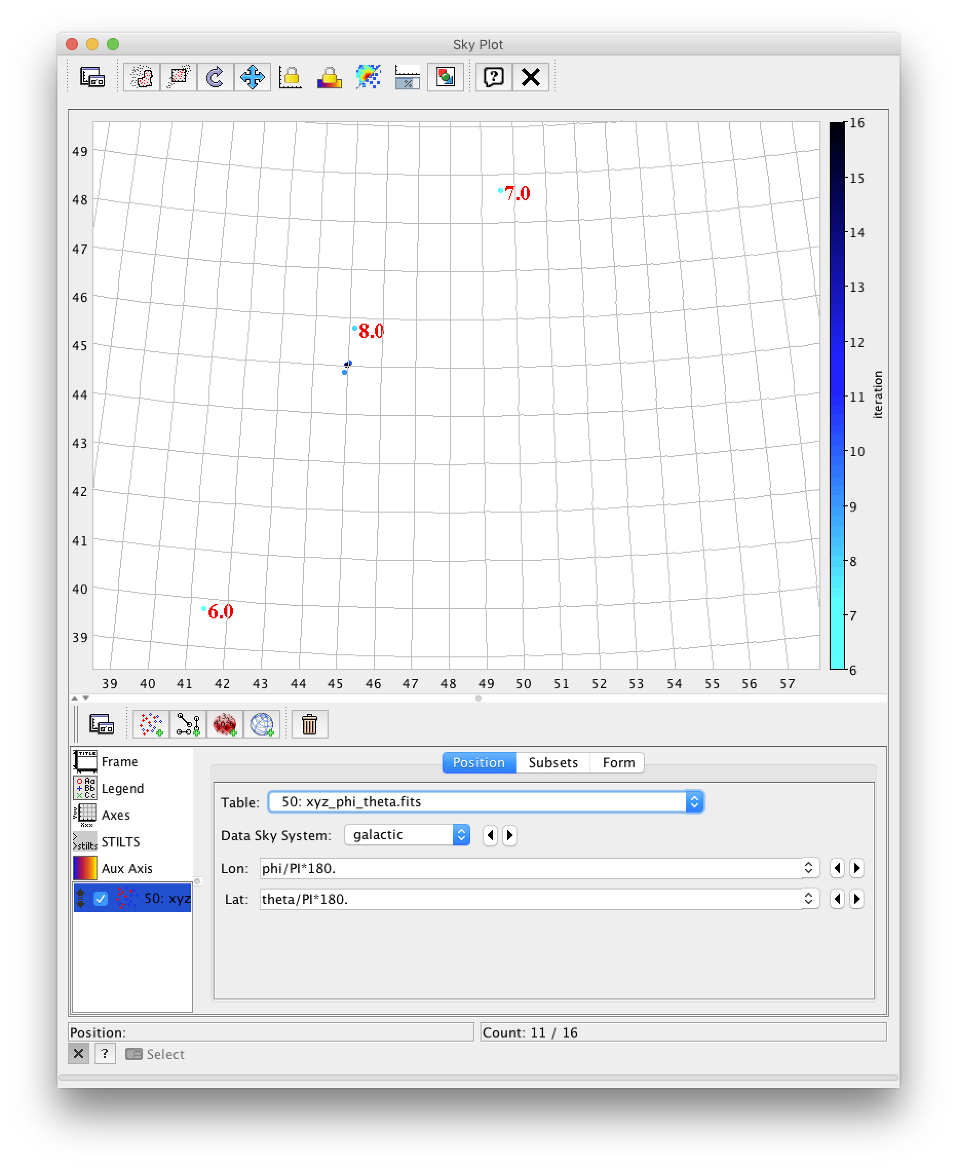
なんとなく大円に沿って探索されているように見える。
(天文のパッケージを利用しているので座標系が銀河座標(galactic)とあるが、これは普通の球座標と同じ。)

収束点付近を拡大。(45 deg, 45 deg)に収束していることがわかる。
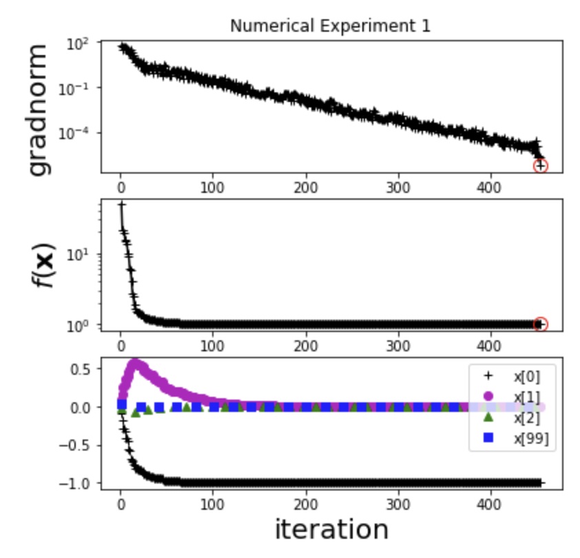
数値実験1(スライド 103 ページ)
_n = 100

diag_matrix_A = np.eye(_n)

for i in range(_n):
    diag_matrix_A[i,i]=i+1

####
array([[  1.,   0.,   0., ...,   0.,   0.,   0.],
       [  0.,   2.,   0., ...,   0.,   0.,   0.],
       [  0.,   0.,   3., ...,   0.,   0.,   0.],
       ...,
       [  0.,   0.,   0., ...,  98.,   0.,   0.],
       [  0.,   0.,   0., ...,   0.,  99.,   0.],
       [  0.,   0.,   0., ...,   0.,   0., 100.]])
import pprint

import numpy
import autograd.numpy as np

from pymanopt.manifolds import Sphere
# from pymanopt.manifolds import Stiefel
from pymanopt import Problem
from pymanopt.solvers import SteepestDescent

from matplotlib import pyplot

global count


# (1) Instantiate a manifold
manifold = Sphere(_n) # (S^2 = 3D points on a 3D sphere)

# (2) Define the cost function (here using autograd.numpy)
def cost(X):

    f = np.dot(np.dot(np.transpose(X),diag_matrix_A), X)

    return f

problem = Problem(manifold=manifold, cost=cost)

# (3) Instantiate a Pymanopt solver


solver = SteepestDescent(logverbosity=2, maxiter=1000)
problem = Problem(manifold, cost, verbosity=0)

print('-'*20)
Xopt, optlog = solver.solve(problem)

print(Xopt)
print('-'*20)

print("Optimization log:")
pprint.pprint(optlog)
fig,axs=pyplot.subplots(3,1, figsize=(6,6))


ax=axs[0]
ax.plot(optlog['iterations']['iteration'],optlog['iterations']['gradnorm'], 'k+')
ax.plot(optlog['iterations']['iteration'],optlog['iterations']['gradnorm'], 'k-')
ax.plot(optlog['iterations']['iteration'][-1], optlog['iterations']['gradnorm'][-1], marker='o', markeredgecolor='r', color='None', markersize=10)

ax.set_ylabel(r'gradnorm',fontsize=20)
ax.set_yscale('log')
ax.set_title('Numerical Experiment 1')


ax=axs[1]
ax.plot(optlog['iterations']['iteration'],optlog['iterations']['f(x)'], 'k+')
ax.plot(optlog['iterations']['iteration'],optlog['iterations']['f(x)'], 'k-')
ax.plot(optlog['iterations']['iteration'][-1], optlog['iterations']['f(x)'][-1], marker='o', markeredgecolor='r', color='None', markersize=10)

ax.set_yscale('log')
ax.set_xlabel('iteration',fontsize=20)
ax.set_ylabel(r'$f({\bf x})$',fontsize=20)


ax=axs[2]
ax.plot(optlog['iterations']['iteration'], numpy.array(optlog['iterations']['x'])[:,0], 'k+', label=r'x[0]')
ax.plot(optlog['iterations']['iteration'], numpy.array(optlog['iterations']['x'])[:,1], 'mo', label=r'x[1]')
ax.plot(optlog['iterations']['iteration'][::14], numpy.array(optlog['iterations']['x'])[::14,2], 'g^', label=r'x[2]')
ax.plot(optlog['iterations']['iteration'][::20], numpy.array(optlog['iterations']['x'])[::20,99], 'bs', label=r'x[99]')

ax.legend(loc='upper right')
ax.set_xlabel('iteration',fontsize=20)
数値実験2(スライド 106 ページ)
_n = 300
_p = 10


diag_matrix_A = np.eye(_n)
diag_matrix_N = np.eye(_p)

for i in range(_n):
    diag_matrix_A[i,i]=i+1

for i in range(_p):
    diag_matrix_N[i,i]=_p-i
diag_matrix_N
####
array([[10.,  0.,  0.,  0.,  0.,  0.,  0.,  0.,  0.,  0.],
       [ 0.,  9.,  0.,  0.,  0.,  0.,  0.,  0.,  0.,  0.],
       [ 0.,  0.,  8.,  0.,  0.,  0.,  0.,  0.,  0.,  0.],
       [ 0.,  0.,  0.,  7.,  0.,  0.,  0.,  0.,  0.,  0.],
       [ 0.,  0.,  0.,  0.,  6.,  0.,  0.,  0.,  0.,  0.],
       [ 0.,  0.,  0.,  0.,  0.,  5.,  0.,  0.,  0.,  0.],
       [ 0.,  0.,  0.,  0.,  0.,  0.,  4.,  0.,  0.,  0.],
       [ 0.,  0.,  0.,  0.,  0.,  0.,  0.,  3.,  0.,  0.],
       [ 0.,  0.,  0.,  0.,  0.,  0.,  0.,  0.,  2.,  0.],
       [ 0.,  0.,  0.,  0.,  0.,  0.,  0.,  0.,  0.,  1.]])
import pprint

import numpy
import autograd.numpy as np

# from pymanopt.manifolds import Sphere
from pymanopt.manifolds import Stiefel
from pymanopt import Problem
from pymanopt.solvers import SteepestDescent

from matplotlib import pyplot

global count


# (1) Instantiate a manifold
manifold = Stiefel(_n,_p) # Stiefel(_p,_n) did not work.

# (2) Define the cost function (here using autograd.numpy)
def cost(X):

    f = np.trace(np.transpose(X) @ diag_matrix_A @ X @ diag_matrix_N)
    #f = np.dot(np.dot(np.transpose(X),diag_matrix_A), X)

    return f

problem = Problem(manifold=manifold, cost=cost)

# (3) Instantiate a Pymanopt solver


solver = SteepestDescent(logverbosity=2, maxiter=100000)
problem = Problem(manifold, cost, verbosity=0)

print('-'*20)
Xopt, optlog = solver.solve(problem)

print(Xopt)
print('-'*20)

# print("Optimization log:")
# pprint.pprint(optlog)
pyplot.clf()

fig,axs=pyplot.subplots(6,1, figsize=(12,12))


ax=axs[0]
ax.set_title('Numerical Experiment 2')

ax.plot(optlog['iterations']['iteration'],optlog['iterations']['gradnorm'], 'k+')
ax.plot(optlog['iterations']['iteration'],optlog['iterations']['gradnorm'], 'k-')
ax.plot(optlog['iterations']['iteration'][-1], optlog['iterations']['gradnorm'][-1], marker='o', markeredgecolor='r', color='None', markersize=10)


ax.axhline(y=10, c='gray')
ax.axhline(y=1, c='gray')
ax.axhline(y=0.1, c='gray')
ax.axhline(y=0.01, c='gray')
ax.axhline(y=0.001, c='gray')
ax.axhline(y=0.0001, c='gray')
ax.set_ylabel(r'gradnorm',fontsize=20)
ax.set_yscale('log')


ax=axs[1]
ax.plot(optlog['iterations']['iteration'],optlog['iterations']['f(x)'], 'k+')
ax.plot(optlog['iterations']['iteration'],optlog['iterations']['f(x)'], 'k-')
ax.plot(optlog['iterations']['iteration'][-1], optlog['iterations']['f(x)'][-1], marker='o', markeredgecolor='r', color='None', markersize=10)

ax.set_yscale('log')
ax.set_xlabel('iteration',fontsize=20)
ax.set_ylabel(r'$f({\bf x})$',fontsize=20)


ax=axs[2]
ax.plot(optlog['iterations']['iteration'], numpy.array(optlog['iterations']['x'])[:,0], 'r-')
ax.set_ylabel('X[:,0]', fontsize=15)

ax=axs[3]
ax.plot(optlog['iterations']['iteration'], numpy.array(optlog['iterations']['x'])[:,1], 'b--')
ax.set_ylabel('X[:,1]', fontsize=15)


ax=axs[4]
ax.plot(optlog['iterations']['iteration'], numpy.array(optlog['iterations']['x'])[:,2], 'm-.')
ax.set_ylabel('X[:,2]', fontsize=15)


ax=axs[5]
ax.plot(optlog['iterations']['iteration'], numpy.array(optlog['iterations']['x'])[:,3], 'g--')
ax.set_ylabel('X[:,3]', fontsize=15)
ax.set_xlabel('iteration',fontsize=20)


pyplot.savefig('Experiment2.png')
