R機械学習/SARIMAXモデルで時系列予測

Introduction

時系列モデリング手法の1つであるSARIMAXをRで実装する方法についてのメモ．

パッケージインストールとインポート

library(xts)  # xts型の提供
library(forecast)  # 時系列モデルの作成と予測
library(ggfortify)  # グラフ描画
library(tidyverse)  # データ操作
library(tseries)  # 正規性の検定

データ操作

今回は，Rにデフォルトで用意されているSeatbeltsデータを使用．

• データ説明：英国における1969年～1984年の自動車運転手の死傷者数．期間中の1983年1月31日にシートベルトの着用が義務づけられた．
• 変数説明
  • DriversKilled：自動車運転手の死亡者数
  • drivers：死傷者数
  • front：前座席の同乗者の死傷者数
  • rear：後部座席の同乗者の死傷者数
  • kms：走行距離
  • PetrolPrice：ガソリン価格
  • VanKilled：バン（軽貨物車）運転者の死亡数
  • law：シートベルトの着用義務

dataset = as.xts(Seatbelts)
dim(dataset)
head(dataset)

Out:

[1] 192   8
       DriversKilled drivers front rear   kms PetrolPrice VanKilled law
1 1969           107    1687   867  269  9059   0.1029718        12   0
2 1969            97    1508   825  265  7685   0.1023630         6   0
3 1969           102    1507   806  319  9963   0.1020625        12   0
4 1969            87    1385   814  407 10955   0.1008733         8   0
5 1969           119    1632   991  454 11823   0.1010197        10   0
6 1969           106    1511   945  427 12391   0.1005812        13   0

データ分割

今回はdriversを自身の過去の値から予測する．説明変数（外生変数）としてkmsとPetroPriceを加える．
シートベルト着用義務の法律が施行される前の期間で訓練データとテストデータを作成する．

dataset_law0 = dataset['::1982-12', c('drivers', 'kms','PetrolPrice')]
train = dataset_law0['::1979-12']
test = dataset_law0['1980-01::']

y_train = train[,'drivers']
X_train = train[,c('kms','PetrolPrice')]
y_test = test[,'drivers']
X_test = test[,c('kms','PetrolPrice')]

データの特徴把握

まずは全変数の時系列グラフを確認

autoplot(train)

Out:

続いて時系列データ特有の特徴を確認

ggtsdisplay(y_train, main = 'drivers')

• 上：データの時系列グラフ
• 左下：自己相関コレログラム；Lag=12で相関が強くなっているため，12ヶ月の周期性があると見て取る．
• 右下：偏自己相関コレログラム；Lag=1で相関が強くなっているため，1時刻前の値が強く影響していると見て取る．
  Out:
  

先ほどとは別の方法でデータの特徴を把握する．
STL分解をすることでデータを以下のように3つの要素に分解する．
$$
元データ=季節性+トレンド+残差
$$

• seasonalグラフ：似た波形が繰り返し出現しているため，季節性ありと判断できる．
• trendグラフ：一部区間で上昇トレンドが見て取れる．
• remainderグラフ：値が極端に高いところなどは外れ値となるが，今回の例では外れ値は無いと判断する．

plot(stl(x=y_train, s.window='periodic'), main='driver')

Out:

モデル作成

SARIMAXモデルは以下のような要素から成るモデル．
$$
SARIMAX = Seasonal(季節成分)+AR(自己回帰)モデル+Integrated(和分)+MA(移動平均)モデル+eXgenous(外因性)
$$

SARIMAXモデルを構築する．
auto.arima()でパラメータを最適化したモデルを自動選択できる．
選択されたパラメータはARIMA(p,d,q)(P,D,Q)[s]の形で表示される．

• p,(P)：ARの次数（季節成分に対するARの次数）
• d,(D)：和分の階数（季節成分に対する和分の階数）
• q,(Q)：MAの次数（季節成分に対するMAの次数）
• s：季節成分の周期

一部引数の詳細

auto.arima(
  y,  # 学習する時系列データ
  max.p = 5,  # 探索する次数p(ARモデル)の最大値
  max.q = 5,  # 探索する次数q(MAモデル)の最大値
  max.P = 2,  # 探索する次数P(季節成分のARモデル)の最大値
  max.Q = 2,  # 探索する次数Q(季節成分のMAモデル)の最大値
  max.order = 5,  #(p+q+P+Q)の合計値．
  seasonal = TRUE,  # TRUE:SARIMAモデル; FALSE:ARIMAモデル
  ic = c("aicc", "aic", "bic"),  # モデル選択に使用される情報量基準
  stepwise = TRUE,  # True:ステップワイズで探索; False:全探索
  trace = FALSE,  # Trueの場合探索したモデルの情報がリスト表示される
  approximation = (length(x) > 150 | frequency(x) > 12),  # 指定した条件に該当する場合近似解を用いる．近似解を使用しない場合はFALSEにする．
  xreg = NULL,  # 外生変数を指定
  parallel = FALSE,  # TRUE:並列処理を行う
  num.cores = 2,  # 並列処理を行う際のコア数の指定
  ...
)

model_sarimax = auto.arima(y_train, max.order=14, ic='aic', ,stepwise=F, parallel=T, num.cores=4, xreg=X_train)
model_sarimax

Out:

Series: y_train 
Regression with ARIMA(3,0,1)(0,1,1)[12] errors 

Coefficients:
          ar1     ar2     ar3     ma1     sma1      kms  PetrolPrice
      -0.5666  0.5975  0.4085  0.9443  -0.8597  -0.0027    -7755.019
s.e.   0.0988  0.0905  0.0885  0.0832   0.1723   0.0197     2259.103

sigma^2 estimated as 16913:  log likelihood=-759.8
AIC=1535.6   AICc=1536.9   BIC=1557.9

ちなみに上記のモデルをArima()を使って構築すると以下のようになる．

model_sarimax2 = arima(y_train, order=c(3,0,1), seasonal=c(0,1,1), xreg=X_train)
model_sarimax2

Out:

Call:
arima(x = y_train, order = c(3, 0, 1), seasonal = c(0, 1, 1), xreg = X_train)

Coefficients:
          ar1     ar2     ar3     ma1     sma1      kms  PetrolPrice
      -0.5666  0.5975  0.4085  0.9443  -0.8597  -0.0027    -7755.019
s.e.   0.0988  0.0905  0.0885  0.0832   0.1723   0.0197     2259.103

sigma^2 estimated as 15926:  log likelihood = -759.8,  aic = 1535.6

モデル評価

残差チェック

checkresidualsで残差に自己相関があるかのチェックを行う．
帰無仮説は「自己相関がない」なので，今回の例では，p-value=0.09であるため，有意水準5%では自己相関があるとは言えないことになる．よってチェックはクリア．
同時に出力されるグラフに関する説明は以下の通り．

• 上：残差のの時系列グラフ；周期性が見られるとそのモデルは信頼性に欠ける
• 左下：残差の自己相関コレログラム；自己相関があるとそのモデルは信頼性に欠ける．
• 右下：残差のヒストグラム；正規分布から逸脱しているとそのモデルは信頼性に欠ける．

checkresiduals(model_sarimax)

Out:

	Ljung-Box test

data:  Residuals from Regression with ARIMA(3,0,1)(0,1,1)[12] errors
Q* = 25.124, df = 17, p-value = 0.09198

Model df: 7.   Total lags used: 24

jarque.bera.test()で残差の正規性の検定を行う．
帰無仮説は「正規分布に従う」なので，今回の例ではp-value=0.6125であるため，有意水準5%では正規分布に従わないとは言えないことになる．よってチェックはクリア．

jarque.bera.test(resid(model_sarimax))

Out:

	Jarque Bera Test

data:  resid(model_sarimax)
X-squared = 0.98046, df = 2, p-value = 0.6125

予測

今回は未来のの外生変数の値が分かっている前提で予測する．

pred_sarimax = forecast(model_sarimax, xreg=X_test, h=length(y_test))
autoplot(pred_sarimax, y_test)

精度評価指標の算出

accuracy(pred_sarimax, y_test)

Out:

                     ME     RMSE       MAE        MPE     MAPE      MASE         ACF1
Training set  -3.552711 120.3265  95.78231 -0.6330721 5.553774 0.6443118 -0.001547839
Test set     -17.228042 147.2290 110.48983 -1.3294291 6.744713 0.7432468           NA

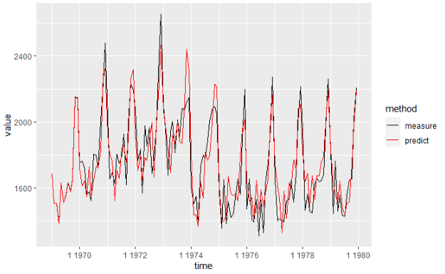
訓練データの実測値と予測値を可視化

test_meas_pred = data.frame(time=index(y_train), measure=as.vector(y_train), predict=model_sarimax$fitted)
test_meas_pred = gather(test_meas_pred, key='method', value='value', -time)

ggplot() +
  geom_line(data=test_meas_pred, aes(x=time, y=value, colour=method)) +
  scale_color_manual(values=c('black', 'red'))

Out:

テストデータの実測値と予測値を可視化

test_meas_pred = data.frame(time=index(y_test), measure=as.vector(y_test), predict=pred_sarimax$mean)
test_meas_pred = gather(test_meas_pred, key='method', value='value', -time)

ggplot() +
  geom_line(data=test_meas_pred, aes(x=time, y=value, colour=method)) +
  scale_color_manual(values=c('black', 'red'))

Out:

モデル比較

モデル単体では精度の良し悪しわ分からないので，今回は以下の3つのモデルで精度を比較する．

• SARIMAXモデル：先ほど作成したもの．
• SARIMAモデル：外生変数を含まないもの．
• ナイーブ予測：モデルを使わないシンプルな予測．今回は1周期前の値をそのまま予測値とする．

SARIMAモデル

model_sarima = auto.arima(y_train, max.order=10, ic='aic', ,stepwise=F, parallel=T, num.cores=4)
model_sarima

Out:

Series: y_train 
ARIMA(1,1,4)(0,1,1)[12] 

Coefficients:
          ar1     ma1      ma2      ma3      ma4     sma1
      -0.7517  0.2348  -0.4050  -0.0433  -0.3153  -0.8690
s.e.   0.1194  0.1455   0.1136   0.0932   0.1028   0.1932

sigma^2 estimated as 17777:  log likelihood=-757.71
AIC=1529.43   AICc=1530.43   BIC=1548.88

pred_sarima = forecast(model_sarima, h=length(y_test))

ナイーブ予測

pred_naive = snaive(y_train, h=length(y_test))

テストデータで実測値と各モデルの予測値を比較

test_meas_pred3 = data.frame(time=index(y_test), measure=as.vector(y_test), SARIMAX=pred_sarimax$mean, SARIMA=pred_sarima$mean, naive=pred_naive$mean)
test_meas_pred3 = gather(test_meas_pred3, key='method', value='value', -time)

ggplot() +
  geom_line(data=test_meas_pred3, aes(x=time, y=value, colour=method)) +
  scale_color_manual(values=c('black', 'blue', 'green', 'red'))

Out:

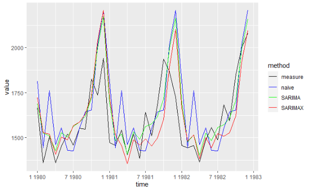
RMSEを比較したところ，テストデータにおいてはSARIMAモデルが最良の結果となった．

rmse_df = rbind(
  t(as.data.frame(accuracy(pred_sarimax, y_test)[,'RMSE'])),
  t(as.data.frame(accuracy(pred_sarima, y_test)[,'RMSE'])),
  t(as.data.frame(accuracy(pred_naive, y_test)[,'RMSE']))
)
rownames(rmse_df) = c('SARIMAX', 'SARIMA', 'naive')
rmse_df

Out:

        Training set Test set
SARIMAX     120.3265 147.2290
SARIMA      123.3607 133.0183
naive       196.8749 182.3017

Conclusion

今回はSARIMAXモデルの構築から精度の評価まで実装してみた．
時系列モデリング手法はVARや状態空間モデル，ディープラーニング等まだまだ気になる手法があるので，それらも随時投稿していこうと思う．

---

---

code

# パッケージインストールとインポート
library(xts)  # xts型の提供
library(forecast)  # 時系列モデルの作成と予測
library(ggfortify)  # グラフ描画
library(tidyverse)  # データ操作
library(tseries)  # 正規性の検定


# データ操作
dataset = as.xts(Seatbelts)
dim(dataset)
head(dataset)

## データ分割
dataset_law0 = dataset['::1982-12', c('drivers', 'kms','PetrolPrice')]
train = dataset_law0['::1979-12']
test = dataset_law0['1980-01::']

y_train = train[,'drivers']
X_train = train[,c('kms','PetrolPrice')]
y_test = test[,'drivers']
X_test = test[,c('kms','PetrolPrice')]

## データの特徴把握
autoplot(train)

ggtsdisplay(y_train, main = 'drivers')

plot(stl(x=y_train, s.window='periodic'), main='driver')


# モデル作成
model_sarimax = auto.arima(y_train, max.order=14, ic='aic', ,stepwise=F, parallel=T, num.cores=4, xreg=X_train)
model_sarimax

model_sarimax2 = arima(y_train, order=c(3,0,1), seasonal=c(0,1,1), xreg=X_train)
model_sarimax2

# モデル評価
## 残差チェック
checkresiduals(model_sarimax)

jarque.bera.test(resid(model_sarimax))

## 予測
pred_sarimax = forecast(model_sarimax, xreg=X_test, h=length(y_test))

autoplot(pred_sarimax, y_test)

accuracy(pred_sarimax, y_test)

test_meas_pred = data.frame(time=index(y_train), measure=as.vector(y_train), predict=model_sarimax$fitted)
test_meas_pred = gather(test_meas_pred, key='method', value='value', -time)

ggplot() +
  geom_line(data=test_meas_pred, aes(x=time, y=value, colour=method)) +
  scale_color_manual(values=c('black', 'red'))

test_meas_pred = data.frame(time=index(y_test), measure=as.vector(y_test), predict=pred_sarimax$mean)
test_meas_pred = gather(test_meas_pred, key='method', value='value', -time)

ggplot() +
  geom_line(data=test_meas_pred, aes(x=time, y=value, colour=method)) +
  scale_color_manual(values=c('black', 'red'))


# モデル比較
model_sarima = auto.arima(y_train, max.order=10, ic='aic', ,stepwise=F, parallel=T, num.cores=4)
model_sarima

pred_sarima = forecast(model_sarima, h=length(y_test))

pred_naive = snaive(y_train, h=length(y_test))

test_meas_pred3 = data.frame(time=index(y_test), measure=as.vector(y_test), SARIMAX=pred_sarimax$mean, SARIMA=pred_sarima$mean, naive=pred_naive$mean)
test_meas_pred3 = gather(test_meas_pred3, key='method', value='value', -time)

ggplot() +
  geom_line(data=test_meas_pred3, aes(x=time, y=value, colour=method)) +
  scale_color_manual(values=c('black', 'blue', 'green', 'red'))

rmse_df = rbind(
  t(as.data.frame(accuracy(pred_sarimax, y_test)[,'RMSE'])),
  t(as.data.frame(accuracy(pred_sarima, y_test)[,'RMSE'])),
  t(as.data.frame(accuracy(pred_naive, y_test)[,'RMSE']))
)
rownames(rmse_df) = c('SARIMAX', 'SARIMA', 'naive')
rmse_df