はじめに
ニュートン法は、
$$f(x)=0$$
を $x$ について解くための反復アルゴリズムです。あるいは、
$$f'(x)=0$$
を解くと極値を求めることができます。今回は関数の極大値を求めてみましょう。
1 変数関数を解く
ニュートン法のアルゴリズムは、
$$x_{n+1}=x_n-\frac{f'(x_n)}{f''(x_n)}$$
です。今回は、
$$f(x)=\frac{\log x}{x^2}$$
の $1<x<5$ における極大値を求めてみましょう。初期値は $x_0=2$ です。
$$f'(x)=\frac{1-2\log x}{x^3}$$
$$f''(x)=\frac{-5+6\log x}{x^4}$$
グラフを見る
import matplotlib.pyplot as plt
import numpy as np

def f(x):
    return np.log(x) / x**2

x = np.linspace(1, 5, 100)
y = f(x)

plt.grid(True)
plt.plot(x, y)
plt.show()

NumPy を使う
1, 2 階の導関数を自力で求めて計算します。
import numpy as np

def df(x):
    return (1 - 2*np.log(x)) / x**3

def ddf(x):
    return (-5 + 6*np.log(x)) / x**4

# 初期値
x = 2

# 要求精度
epsilon = 1e-5

print("n\tx\tdf(x)")
n = 1

while abs(df(x)) > epsilon:
    # xの更新
    x = x - df(x)/ddf(x)

    print("{}\t{:.5f}\t{:.5f}".format(n, x, df(x)))
    n += 1

print("x = %f" % x)
結果
n       x       df(x)
1       1.08147 0.66675
2       1.28281 0.23775
3       1.46646 0.07429
4       1.59358 0.01681
5       1.64277 0.00163
6       1.64865 0.00002
7       1.64872 0.00000
x = 1.648721
PyTorch を使う
PyTorch を使えば、微分値の計算を自動でやってくれます。
import torch
from torch.func import hessian, jacfwd

def f(x):
    return torch.log(x) / x**2

# 初期値
x = 2
x = torch.tensor(x, dtype=torch.float64)

# 要求誤差
epsilon = 1e-5

print("n\tx\tdf(x)")
n = 1

df = jacfwd(f)
ddf = hessian(f)

while abs(df(x)) > epsilon:
    # xの更新
    x = x - df(x)/ddf(x)

    print("{}\t{:.5f}\t{:.5f}".format(n, x.item(), df(x).item()))
    n += 1

print("x = %f" % x.item())
結果
n       x       df(x)
1       1.08147 -0.04829
2       1.28281 0.66675
3       1.46646 0.23775
4       1.59358 0.07429
5       1.64277 0.01681
6       1.64865 0.00163
7       1.64872 0.00002
8       1.64872 0.00000
x = 1.648721
| 関数名 | 説明 |
|---|---|
torch.tensor() |
テンソルの作成 |
SciPy を使う
SciPy を使えばもっと簡単に解けます。(本当は scipy.optimize.minimize() を使うべきですが。)
import numpy as np
from scipy.optimize import newton, approx_fprime

def f(x):
    return np.log(x) / x**2

def df(x):
    return approx_fprime(x, f)

x = newton(df, 2)
print("x = %f" % x.item())
結果
x = 1.648721
多変数関数を解く
アルゴリズムは、
$$x_{n+1}=x_n-H^{-1}J$$
です。
今回は、
$$ f(x_0,x_1) = \frac{\log x_0}{x_0^2} - \frac{x_1^2}{37} + \frac{x_1}{7}$$
の $x_0=2, x_1=2$ 付近の極値を求めてみましょう。
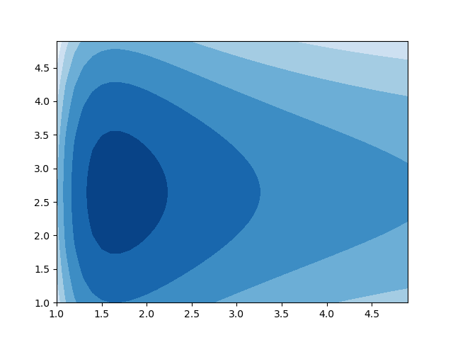
グラフを見る
import matplotlib.pyplot as plt
import numpy as np

def f(x):
    return np.log(x[0])/x[0]**2 - x[1]**2 / 37 + x[1]/7

x0 = np.arange(1, 5, 0.1)
x1 = np.arange(1, 5, 0.1)
x0, x1 = np.meshgrid(x0, x1)

y = f([x0, x1])

plt.contourf(x0, x1, y, cmap='Blues')
plt.show()
PyTorch を使う
import torch
from torch.func import hessian, jacfwd
from torch.linalg import solve

def f(x):
    return torch.log(x[0])/x[0]**2 - x[1]**2/37 + x[1]/7

# 初期値
x = [2, 2]
x = torch.tensor(x, dtype=torch.float64)

# 要求誤差
epsilon = 1e-5

print("n\tx0\tx1\tdf0(x)\tdf1(x)")
n = 1

J = jacfwd(f)
H = hessian(f)

while J(x).sum().abs() > epsilon:
    # xの更新
    x = x - solve(H(x), J(x))

    print("{}\t{:.5f}\t{:.5f}\t{:.5f}\t{:.5f}".format(n,
        x[0].item(), x[1].item(), J(x)[0].item(), J(x)[1].item()))
    n += 1

print("x0 = %f, x1 = %f" % (x[0].item(), x[1].item()))
結果
n       x0      x1      df0(x)  df1(x)
1       1.08147 2.64286 0.66675 0.00000
2       1.28281 2.64286 0.23775 0.00000
3       1.46646 2.64286 0.07429 0.00000
4       1.59358 2.64286 0.01681 0.00000
5       1.64277 2.64286 0.00163 0.00000
6       1.64865 2.64286 0.00002 0.00000
7       1.64872 2.64286 0.00000 0.00000
x0 = 1.648721, x1 = 2.642857
SciPy を使う
import numpy as np
from scipy.optimize import newton, approx_fprime

def f(x):
    return np.log(x[0])/x[0]**2 - (x[1]**2)/37 + x[1]/7

def df(x):
    return approx_fprime(x, f)

x = newton(df, [2, 2])
print("x0 = %f, x1 = %f" % (x[0].item(), x[1].item()))
結果
x0 = 1.648721, x1 = 2.642857
参考