はじめに
疎行列とは、行列の要素の大部分が0である行列のことを言います。数値計算や機械学習、グラフ理論など幅広い分野で扱われている(と思います)。行列内のほとんどが0という特徴から、0を無視する工夫をすれば、高速に行列計算を実施することが可能になります。例えば、9割近くが0の大規模疎行列(100万行×100万列とか)で非ゼロ部分だけ用いて計算すれば、計算時間が約1/10になり計算が早く終わらせることが可能になることが容易に想像できます。つまり、工夫すれば、1反復あたりの計算量を$O(N^2)$から$O(N)$に落として計算することが可能になります。
本記事では、Python・Numpy・Scipyを用いて、こうした疎行列計算について解説していきます。追加したいことが出てきたら適宜更新していきます。間違い等ございましたら、コメントにてご連絡して頂けたら幸いです。
対象読者
- Pythonを扱える人
- 行列計算に興味がある人
概要
疎行列計算をPythonで扱う上で必要な概念をまとめた後、直接法・反復法のライブラリについて言及します。最終的に前回記事で作成した問題を非定常反復法と呼ばれる手法で解きます。
使用するライブラリ:Scipy・Numpy・matplotlib
計算結果

記事内目次
1. 疎行列
1-1. 密行列と疎行列
-
密行列
密な行列。行列内に0がほとんどない行列。数学の問題とかで、おそらくこちらの方が見慣れている人が多いかも。
  \left(
    \begin{array}{cccc}
      2  & 1 &  1 & \ldots  & \ldots & 1 \\
      1 & 2  & -1 & 1 & \ldots & 1 \\
      1  & 1 & 2  & 1 & 1 & \vdots  \\
      \vdots & \ddots & \ddots & \ddots & \ddots & \vdots\\
      1  & 1 & \ddots & 1 & 2  & 1 \\
      1  & 1 & \ldots & 1 & 1 & 2
    \end{array}
  \right)
-
疎行列
疎(まば)らな行列。単に行列内に0がたくさんあるってだけ。0が関係する計算の部分を工夫すれば、ほとんど計算しなくて済むため、特殊な手法で計算する。本記事で扱う。
  \left(
    \begin{array}{cccc}
      2  & -1 &  0 & \ldots  & \ldots & 0 \\
      -1 & 2  & -1 & 0 & \ldots & 0 \\
      0  &-1 & 2  & -1 & \ddots & \vdots  \\
      \vdots & \ddots & \ddots & \ddots & \ddots & 0\\
      0  & 0 & \ddots & -1 & 2  & -1 \\
      0  & 0 & \ldots & 0 & -1 & 2
    \end{array}
  \right)
1-2. 疎行列の可視化
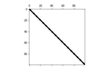
疎行列の可視化には、matplotlibのspy関数を用いるのが一番だと思います。これは行列で0の部分は白色、何か数が入っている場合は色付きで表示してくれます。
上の疎行列が$100 \times 100$の行列だとすると、以下のようになります。
2. 疎行列の格納形式
0を無視して疎行列を扱うために、特殊な方式を用いて疎行列を表現します。こうすることにより、使用するメモリや計算量などを大幅に削減することが可能になります。よくわからないかもしれないので、下に示す行列を用いながら説明します。ただし、a=1, b=2, c=3, d=4, e=5, f=6とします。
  \left(
    \begin{array}{cccc}
      a & 0 & 0 & 0 & 0 & 0 \\
      b & 0 & 0 & 0 & 0 & 0 \\
      0 & 0 & 0 & c & 0 & d \\
      0 & 0 & 0 & 0 & 0 & 0 \\
      0 & 0 & 0 & 0 & e & 0 \\
      0 & 0 & 0 & 0 & 0 & f
    \end{array}
  \right)
2-1. リストのリスト(List of Lists : LIL)
行ごとに、(列,要素)のタプルを格納します。
最初に行列にデータを格納する際は、LIL方式を用いるのが楽です。その後、下で示すCRSやCCS方式に変換するのがわかりやすくて良いと思います。PythonのlistやNumpyのarrayの操作に慣れてたら、そんなに難しくないです。上の例だと、
| 行 | (列, 要素) |
|---|---|
| 0 | (0, a) |
| 1 | (0, b) |
| 2 | (3, c), (5, d) |
| 4 | (4, e) |
| 5 | (5, f) |
という形で格納され、少ないメモリで疎行列を記述できることがわかります。大規模な疎行列になればなるほど、こうした0を無視する格納方式の良さが出てきます。
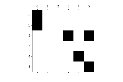
scipy.sparse.lil_matrix
scipyで用意されているLIL形式を扱うための関数lil_matrix。行列の非ゼロ要素の入力が楽に行えるため、疎行列を生成する際によく用いられることが多いです。
from scipy.sparse import lil_matrix

# Create sparse matrix
a=lil_matrix((6,6))

# Set the non-zero values
a[0,0]=1.; a[1,0]=2.; a[2, 3]=3.; a[2, 5]=4.; a[4, 4]=5.; a[5, 5]=6.

print("(row, column) value")
print(a, "\n")
print("Normal type: ")
print(a.todense())  # 普通の行列の形に戻す
print("LIL type: ")
print(a.rows)  # 各行で何列目に非ゼロ要素が入っているか
print(a.data)  # 各行での非ゼロ要素
実行結果は以下の通り。
(row, column) value
  (0, 0)	1.0
  (1, 0)	2.0
  (2, 3)	3.0
  (2, 5)	4.0
  (4, 4)	5.0
  (5, 5)	6.0

Normal type:
[[1. 0. 0. 0. 0. 0.]
 [2. 0. 0. 0. 0. 0.]
 [0. 0. 0. 3. 0. 4.]
 [0. 0. 0. 0. 0. 0.]
 [0. 0. 0. 0. 5. 0.]
 [0. 0. 0. 0. 0. 6.]]

LIL type:
[list([0]) list([0]) list([3, 5]) list([]) list([4]) list([5])]
[list([1.0]) list([2.0]) list([3.0, 4.0]) list([]) list([5.0]) list([6.0])]
2-2. 圧縮行格納方式(Compressed Sparse Row: CSR)
CRS(Compressed Row Storage)と呼ぶ人もいる。行方向に探索し、非ゼロの行列の要素を格納していく。わかりにくい場合は、東京大学の中島先生の資料をお読みください。対角成分を除外してCSR方式を実行する例が示されております。
CSR方式を用いると、
  \left(
    \begin{array}{cccc}
      a & 0 & 0 & 0 & 0 & 0 \\
      b & 0 & 0 & 0 & 0 & 0 \\
      0 & 0 & 0 & c & 0 & d \\
      0 & 0 & 0 & 0 & 0 & 0 \\
      0 & 0 & 0 & 0 & e & 0 \\
      0 & 0 & 0 & 0 & 0 & f
    \end{array}
  \right)
は、
- indices:
IA = [0, 0, 3, 5, 4, 5]- 上の行から順に要素が何列目にあるかを表示している。indicesのサイズは非ゼロ要素の数となります。
- data:
A = [a, b, c, d, e, f]- indicesに合わせて、その非ゼロの要素を示す。dataはindicesと同じサイズになります。
- indptr:
IN = [0, 1, 2, 4, 4, 5, 6]- 各行で要素が何個あるかを数えて、それを積算した値を示す。0から始まるため、行数+1のサイズになります。
の3つのリストで表現することが可能です。こちらも、少ないメモリで疎行列を記述できることがわかります。疎行列計算を行う際は、このCSR形式を用いることが多いと思います。如何に早く計算が終わるのかは、3章の四則演算のところで述べてます。
これらのリストが何を表すのかを示すために、indicesを元の行列の要素の下付き文字、indptrを右側に示すと以下のようになります。
  \left(
    \begin{array}{cccccc|c}
      col0    & col1   & col2  &  col3   & col4  & col5 & indptr  \\
          &   &   &     &   & & 0 \\
      a_0 & 0 & 0 & 0   & 0 & 0 & 1 \\
      b_0 & 0 & 0 & 0   & 0 & 0 & 2 \\
      0   & 0 & 0 & c_3 & 0 & d_5& 4 \\
      0   & 0 & 0 & 0   & 0 & 0 & 4 \\
      0   & 0 & 0 & 0   & e_4 & 0 & 5 \\
      0   & 0 & 0 & 0   & 0 & f_5 & 6
    \end{array}
  \right)
考え方をこの例を用いながら説明すると、
- 初期状態
indices: IA = []data: A = []-
indptr: IN = [0, 0, 0, 0, 0, 0, 0](行数+1のサイズ)とします。
- 0行目
- 0列目から順に非ゼロ要素がないかを探索します。
- aを発見!Aに要素aを追加。
- aは0列目にあるため、IAに0を追加。
- 0行目では要素を1つ見つけたため、
IN[1]に1を追加します。 IA = [0], A = [a], IN = [0, 1, 0, 0, 0, 0, 0]
- 1行目
- 0列目から順に非ゼロ要素がないかを探索します。
- bを発見!Aに要素bを追加。
- bは0列目にあるため、IAに0を追加。
- 1行目では要素を1つ見つけたため、
IN[2]に1+IN[1]を追加します。 IA = [0, 0], A = [a, b], IN = [0, 1, 2, 0, 0, 0, 0]
- 2行目以降、これを繰り返します。
IA = [0, 0, 3, 5, 4, 5], A = [a, b, c, d, e, f], IN = [0, 1, 2, 4, 4, 5, 6]
scipy.sparse.csr_matrix
scipyで用意されているCSR形式を扱うための関数csr_matrix。scipy.sparse.csr_matrix(mtx)のように任意の行列mtxを入れれば、CSR形式に直してくれます。mtxの形式は、list、numpy.ndarray、numpy.matrixなどです。LIL形式からCSR形式にする際は、tocsr()を用いれば良いです。
a_csr = a.tocsr()
print("Normal type: ")
print(a_csr.todense())
print("csr type:")
print(a_csr.indices)
print(a_csr.data)
print(a_csr.indptr)
Normal type:
[[1. 0. 0. 0. 0. 0.]
 [2. 0. 0. 0. 0. 0.]
 [0. 0. 0. 3. 0. 4.]
 [0. 0. 0. 0. 0. 0.]
 [0. 0. 0. 0. 5. 0.]
 [0. 0. 0. 0. 0. 6.]]

csr type:
[0 0 3 5 4 5]  # indices: 上の行から順に要素が何列目にあるかを表示している。
[1. 2. 3. 4. 5. 6.]  # data: indicesに合わせて、その非ゼロの要素を示す。
[0 1 2 4 4 5 6]  # indptr: 各行で要素が何個あるかを数えて、それを積算する。0から始まるため、行数+1のサイズになる。
2-3. 圧縮列格納方式(Compressed Sparse Column: CSC)
CCSと呼ぶ人もいる。列方向に探索し、非ゼロの行列の要素を格納していく。CSR方式の列バージョン。
scipy.sparse.csc_matrix
scipyで用意されているCSC形式を扱うための関数csc_matrix。scipy.sparse.csc_matrix(mtx)のように任意の行列mtxを入れれば、CSC形式に直してくれます。mtxの形式は、list、numpy.ndarray、numpy.matrixなどです。LIL形式からCSC形式にする際は、tocsc()を用いれば良いです。
a_csc = a.tocsc()
print("Normal type: ")
print(a_csc.todense())
print("csc type:")
print(a_csc.indices)
print(a_csc.data)
print(a_csc.indptr)
Normal type:
[[1. 0. 0. 0. 0. 0.]
 [2. 0. 0. 0. 0. 0.]
 [0. 0. 0. 3. 0. 4.]
 [0. 0. 0. 0. 0. 0.]
 [0. 0. 0. 0. 5. 0.]
 [0. 0. 0. 0. 0. 6.]]

csc type:
[0 1 2 4 2 5]  # indices: 左の列から順に要素が何行目にあるかを表示している。
[1. 2. 3. 5. 4. 6.]  # data: indicesに合わせて、その非ゼロの要素を示す。
[0 2 2 2 3 4 6]  # indptr: 各列で要素が何個あるかを数えて、それを積算する。0から始まるため、列数+1のサイズになる。
2-4. その他
他にも色々な行列格納方式があるので、詳しく知りたい方はWikipedia等をご覧ください。
3. 四則演算など
疎行列の計算をする際は、CSR方式かCSC方式で格納した後に計算を行うのが、最も一般的です。慣れ親しんでいるnumpyの四則演算と同じように実行することが可能です。
# csr example
# Create sparse matrix
a = scipy.sparse.lil_matrix((6,6))
# Set the non-zero values
a[0,0]=1.; a[1,0]=2.; a[2, 3]=3.; a[2, 5]=4.; a[4, 4]=5.; a[5, 5]=6.
a_csr = a.tocsr()
a_matrix = a.todense()

b = np.arange(6).reshape((6,1))
print(b)
print(a_matrix * b)
print(a_csr * b)
print(a_matrix.dot(b))
print(a_csr.dot(b))
CSR形式で格納した疎行列同士の掛け算もこんな感じで計算可能。
b_sparse = scipy.sparse.lil_matrix((6,6))
b_sparse[0,1]=1.; b_sparse[3,0]=2.; b_sparse[3, 3]=3.; b_sparse[5, 4]=4.
b_csr = b_sparse.tocsr()
print(b_csr.todense())
print(a_matrix * b_csr)
print((a_csr * b_csr).todense())
これらを踏まえ、CSR(圧縮行格納)方式の有効性を確認してみましょう。以下のコードをJupyter notebook上で実行してみてください。普通の行列を用いて解くよりCSR方式の方が相当(1000倍くらい)早く計算が終わるのがわかると思います。
import scipy.sparse
import numpy as np
import matplotlib.pyplot as plt
num = 10**4
# Creat LIL type sparse matrix
a_large = scipy.sparse.lil_matrix((num,num))
# Set the non-zero values
a_large.setdiag(np.ones(num)*2)
a_large.setdiag(np.ones(num-1)*-1, k=1)
a_large.setdiag(np.ones(num-1)*-1, k=-1)
a_large_csr = a_large.tocsr()
a_large_dense = a_large.todense()
plt.spy(a_large_csr)
b = np.ones(num)
%timeit a_large_csr.dot(b)  # CSR方式
%timeit a_large_dense.dot(b)  # 普通の行列
注意点
np.dot(a_csr, b)のようにnumpyのdot関数の引数にcsr形式の行列を入れてしまうと、
[[<6x6 sparse matrix of type '<class 'numpy.float64'>'
	with 6 stored elements in Compressed Sparse Row format>]
 [<6x6 sparse matrix of type '<class 'numpy.float64'>'
	with 6 stored elements in Compressed Sparse Row format>]
 [<6x6 sparse matrix of type '<class 'numpy.float64'>'
	with 6 stored elements in Compressed Sparse Row format>]
 [<6x6 sparse matrix of type '<class 'numpy.float64'>'
	with 6 stored elements in Compressed Sparse Row format>]
 [<6x6 sparse matrix of type '<class 'numpy.float64'>'
	with 6 stored elements in Compressed Sparse Row format>]
 [<6x6 sparse matrix of type '<class 'numpy.float64'>'
	with 6 stored elements in Compressed Sparse Row format>]]
のようになりうまく計算できません。
4. Matrix Market 形式
本記事では使用しませんが、疎行列の表現の一つであるMatrix Market形式についても言及しておきます。疎行列のデータは、この形式かRutherford Boeingという形式で基本的には配布されており、疎行列計算に関する論文や実装などを参照しようとすると必要な知識になります。
疎行列問題のデータセットとしては、The SuiteSparse Matrix Collection formerly the University of Florida Sparse Matrix Collectionが有名かと思います。
  \left(
    \begin{array}{cccc}
      a & 0 & 0 & 0 & 0 & 0 \\
      b & 0 & 0 & 0 & 0 & 0 \\
      0 & 0 & 0 & c & 0 & d \\
      0 & 0 & 0 & 0 & 0 & 0 \\
      0 & 0 & 0 & 0 & e & 0 \\
      0 & 0 & 0 & 0 & 0 & f
    \end{array}
  \right)
をMatrix Market(MM)形式で表すと
%%MatrixMarket matrix coordinate real general
%=================================================================================
%
% This ASCII file represents a sparse MxN matrix with L
% nonzeros in the following Matrix Market format:
%
% +----------------------------------------------+
% |%%MatrixMarket matrix coordinate real general | <--- header line
% |%                                             | <--+
% |% comments                                    |    |-- 0 or more comment lines
% |%                                             | <--+
% |    M  N  L                                   | <--- rows, columns, entries
% |    I1  J1  A(I1, J1)                         | <--+
% |    I2  J2  A(I2, J2)                         |    |
% |    I3  J3  A(I3, J3)                         |    |-- L lines
% |        . . .                                 |    |
% |    IL JL  A(IL, JL)                          | <--+
% +----------------------------------------------+
%
% Indices are 1-based, i.e. A(1,1) is the first element.
%
%=================================================================================
  6  6  6
    1     1   a
    2     1   b
    3     4   c
    5     5   e
    3     6   d
    6     6   f
となります。上のコメントを見ればわかると思います。
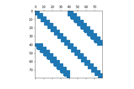
この記事がわかりやすいです。とりあえず適当に選んだsteam3という疎行列で色々遊んでみます。
Matrix market形式を読み込む際にはscipy.ioを用います。
-
scipy.io.mminfoを実行すると、何行何列の行列で、非ゼロの要素が何個あるかなどを教えてくれます。 -
scipy.io.mmreadでMatrix Market形式の行列を読み込むことが可能です。返り値は、numpy.arrayかcoo_matrix形式(csr格納形式と似たようなものです)です。
import scipy.io as io
print(io.mminfo("steam3/steam3.mtx"))
steam3 = io.mmread("steam3/steam3.mtx").tocsr()
print(steam3.todense())
plt.spy(steam3)
(80, 80, 928, 'coordinate', 'real', 'general')
matrix([[-3.8253876e+05,  0.0000000e+00,  0.0000000e+00, ...,
          0.0000000e+00,  0.0000000e+00,  0.0000000e+00],
        [ 9.1147205e-01, -9.5328382e+03,  0.0000000e+00, ...,
          0.0000000e+00,  0.0000000e+00,  0.0000000e+00],
        [ 0.0000000e+00,  0.0000000e+00, -2.7754141e+02, ...,
          0.0000000e+00,  0.0000000e+00,  0.0000000e+00],
        ...,
        [ 0.0000000e+00,  0.0000000e+00,  0.0000000e+00, ...,
         -4.6917325e+08,  0.0000000e+00, -1.2118734e+05],
        [ 0.0000000e+00,  0.0000000e+00,  0.0000000e+00, ...,
          0.0000000e+00, -1.3659626e+07,  0.0000000e+00],
        [ 0.0000000e+00,  0.0000000e+00,  0.0000000e+00, ...,
          2.1014810e+07, -3.6673643e+07, -1.0110894e+04]])
5. 直接法ライブラリ
scipy.sparse.linalg.dsolveの中に入っています。前の記事で解いたAx=bという問題(詳しくは下の式参照)を例に実装しました(実装はほぼ変わっていません)。
  \left(
    \begin{array}{cccc}
      2 \left(\frac{1}{d} + 1 \right) & -1 &  0 & \ldots  & \ldots & 0 \\
      -1 & 2 \left(\frac{1}{d} + 1 \right) & -1 & 0 & \ldots & 0 \\
      0  &-1 & 2 \left(\frac{1}{d} + 1 \right) & -1 & 0 & \ldots  \\
      \vdots & \ddots & \ddots & \ddots & \ddots & \ddots\\
      0  & 0 & \ddots & -1 & 2 \left(\frac{1}{d} + 1 \right) & -1 \\
      0  & 0 & \ldots & 0 & -1 & 2 \left(\frac{1}{d} + 1 \right)
    \end{array}
  \right)
  \left(
    \begin{array}{c}
      T_1^{n+1}  \\
      T_2^{n+1}  \\
      T_3^{n+1}    \\
      \vdots \\
      T_{M-1}^{n+1} \\
      T_M^{n+1}
    \end{array}
  \right)
   =
   \left(
    \begin{array}{c}
      T_2^{n} + 2 \left(\frac{1}{d} - 1 \right) T_1^{n} + \left(T_0^n + T_0^{n+1}\right) \\
      T_3^{n} + 2 \left(\frac{1}{d} - 1 \right) T_2^{n} + T_1^n  \\
      T_4^{n} + 2 \left(\frac{1}{d} - 1 \right) T_3^{n} + T_2^n  \\
      \vdots \\
      T_M^{n} + 2 \left(\frac{1}{d} - 1 \right) T_{M-1}^{n} + T_{M-2}^n  \\
      \left(T_{M+1}^n + T_{M+1}^{n+1}\right) + 2 \left(\frac{1}{d} - 1 \right) T_{M}^{n} + T_{M-1}^n
    \end{array}
  \right)
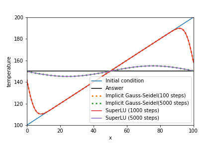
デフォルトの設定では、scipy.sparse.linalg.dsolve(csr形式のA行列, bベクトル)でSuperLU分解が行われるはずです。
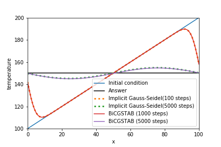
定常反復法のガウス・ザイデル法と比較結果が下の画像です。
import numpy as np
import matplotlib.pyplot as plt
import scipy.sparse
# Make stencils
# Creat square wave
Num_stencil_x = 101
x_array = np.float64(np.arange(Num_stencil_x))
temperature_array = x_array + 100
temperature_lower_boundary = 150
temperature_upper_boundary = 150
Time_step = 100
Delta_x = max(x_array) / (Num_stencil_x-1)
C = 1
Delta_t = 0.2
kappa = 0.5
d = kappa * Delta_t / Delta_x**2
total_movement = C * Delta_t * (Time_step+1)
exact_temperature_array = (temperature_upper_boundary - temperature_lower_boundary) / (x_array[-1] - x_array[0]) * x_array + temperature_lower_boundary
plt.plot(x_array, temperature_array, label="Initial condition")
print("Δx:", Delta_x, "Δt:", Delta_t, "d:", d)

temperature_sp = temperature_array.copy()
for n in range(Time_step):
    a_matrix = np.identity(len(temperature_sp)) * 2 *(1/d+1) \
                - np.eye(len(temperature_sp), k=1) \
                - np.eye(len(temperature_sp), k=-1)
    temp_temperature_array = np.append(np.append(
                        temperature_lower_boundary,
                        temperature_sp), temperature_upper_boundary)
    b_array = 2 * (1/d - 1) * temperature_sp + temp_temperature_array[2:] + temp_temperature_array[:-2]
    b_array[0] += temperature_lower_boundary
    b_array[-1] += temperature_upper_boundary
    a_csr = scipy.sparse.csr_matrix(a_matrix)
    temperature_sp = spla.dsolve.spsolve(a_csr, b_array)
plt.plot(x_array, temperature_sp, label="SuperLU")
plt.legend(loc="lower right")
plt.xlabel("x")
plt.ylabel("temperature")
plt.xlim(0, max(x_array))
plt.ylim(100, 200)
6. 反復法ライブラリ
非定常反復法のライブラリがscipyでは実装されております。scipy.sparse.linalg.isolveの中に入っております。非定常反復法がよくわからない人は前の記事をご覧ください。使用できるライブラリの一部を以下に列挙しておきます。これら以外のライブラリを使いたい場合は、Scipyのマニュアルから探してみてください。
- 対称行列
-
cg共役勾配法(Conjugate Gradient method : CG法) - 正定値対称行列のみ -
minres最小残差法(MINimum RESidual: MINRES法)
-
- 非対称行列
-
bicg双共役勾配法(Bi-Conjugate Gradient: BiCG法) -
cgs自乗共役勾配法(Conjugate Residual Squared: CGS法) -
bicgstab双共役勾配安定化法(BiCG Stabilization: BiCGSTAB法) -
gmres一般化最小残差法(Generalized Minimal Residual: GMRES法) -
qmr準最小残差法(Quasi-Minimal Residual: QMR法)
-
直接法で使用した同じ問題に対して、BiCGSTAB法での実装例とその実行結果を以下に示します。
temperature_sp = temperature_array.copy()
for n in range(Time_step):
    a_matrix = np.identity(len(temperature_sp)) * 2 *(1/d+1) \
                - np.eye(len(temperature_sp), k=1) \
                - np.eye(len(temperature_sp), k=-1)
    temp_temperature_array = np.append(np.append(
                        temperature_lower_boundary,
                        temperature_sp), temperature_upper_boundary)
    b_array = 2.0 * (1/d - 1.0) * temperature_sp + temp_temperature_array[2:] + temp_temperature_array[:-2]
    b_array[0] += temperature_lower_boundary
    b_array[-1] += temperature_upper_boundary
    a_csr = scipy.sparse.csr_matrix(a_matrix)
    temperature_sp = spla.isolve.bicgstab(a_csr, b_array)[0]
plt.plot(x_array, temperature_sp, label="Scipy.isolve (1000 steps)")

plt.legend(loc="lower right")
plt.xlabel("x")
plt.ylabel("temperature")
plt.xlim(0, max(x_array))
plt.ylim(100, 200)
まとめ
- 疎行列には0を無視する格納方式がある
- LIL方式は疎行列を作成するときに用いることが多い。
- CSR方式とCSC方式は疎行列計算をするときに用いることが多い。
- CSR方式で計算すると、普通の行列の形で計算するより、圧倒的に早く計算が終わることが確認できた。
- Matrix Market方式で疎行列は配布されることが多い。
- 直接法と非定常反復法の関数がScipyに実装されており、簡単に使用することができる。
という感じかと思います。