ライブラリなしでSNEをゼロから実装！Pythonで学ぶ次元圧縮

記事について

• t-SNEのベースとなったSNEについて、勉強してライブラリを使わずに実装したので、その時の備忘メモ。
• 数式的な説明の細かいところは、こちらの参考ページを見ていただいたほうが良いかもしれません。
  • 参考ページ：https://qiita.com/g-k/items/120f1cf85ff2ceae4aba

概要

• 次元圧縮方法である。
• t-SNEのベースとなった手法。
• 高次元空間での局所的な構造を維持したまま、低次元空間で表現する。

考え方

• 高次元空間のデータを $\mathbf{X}$ とする。 そしてこれを低次元空間で表現したときの点を $\mathbf{Y}$として記述する。

• あるデータサンプル $\mathbf{x}_i$ に注目する。このとき、 $\mathbf{x}_j$ との類似度を以下のように考えて、定量化する

  • 『$\mathbf{x}_i$ が与えられたときに、近傍として $\mathbf{x}_j$ を選択する条件付き確率』として類似度を捉える。

  • その条件付き確率を $p_{j|i}$ と表現する。 SNEの場合は、確率分布として正規分布を採用しているので、以下のように定式化される。

    p_{j|i} = \frac
    {exp(- \frac{(\mathbf{x}_i-\mathbf{x}_j)^2}{2\sigma_i^2} )}
    {\sum_{k \neq i} exp(- \frac{(\mathbf{x}_i-\mathbf{x}_k)^2}{2\sigma_i^2} )}
    

  • 補足①：多次元正規分布の場合、共分散行列を使うのではないかと思うかもしれないが、SNEの場合は、等方分布を仮定した手法となっているため、今回はこれでOK。

    • 拡張版として、共分散行列でやる方法もある模様。
    • 等方的な正規分布を仮定しているのは、SNEではあくまでも局所的な距離構造を再現することに重きをおいているため、いま注目している点 $\mathbf{x}_i$ からの距離を考えるための分布として等方分布が適している、ということがある。
    • さらに、等方的な正規分布を仮定したほうが（共分散行列を計算するよりも）計算量が少なくて済むので、実装面も楽である。

  • 補足②：正規分布なので、正確に記載すると、以下のように記載すべきだが、分母分子で打ち消しあうので、記載していない。

  p_{j|i} = \frac
  {\frac{1}{\sqrt{2 \pi \sigma_i^2}}   exp(- \frac{(\mathbf{x}_i-\mathbf{x}_j)^2}{2\sigma_i^2} )}
  {\sum_{k \neq i} \frac{1}{\sqrt{2 \pi \sigma_i^2}} exp(- \frac{(\mathbf{x}_i-\mathbf{x}_k)^2}{2\sigma_i^2} )}
  

  • 補足③： $p_{j|i}$ の計算式のうち、 $\sigma_i$ が未定のままである。これは分析者が指定するperplexityに応じて、アルゴリズムで自動的に決まる数値である。 perplexityはハイパーパラメータなので、分析者がいろいろ試すことになる（ちなみに、一般的には5.0~50.0くらいにするらしい）。

    • 分析者が決めた $perplexity$ を満たすように、以下の等式で計算していく。

    perplexity = 2^{H(p_i)}
    

    H(p_i) = - \sum p_{j|i} \times log( p_{j|i})
    

    • したがって、 $\sigma_i$ はデータサンプルの数だけ存在する。

• 高次元空間の構造を低次元でどれくらい再現できているかを表す指標として（逆を言えば、どれくらい似ていないかを表す指標）として、KLダイバージェンスを利用する。

Loss = \sum_i KL(P_i||Q_i) = \sum_i \{  \sum_j p_{j|i} (log(\frac{p_{j|i}}{q_{j|i}}))\}

• これを最小化するように、確率的勾配法で $\mathbf{y}_i$ を最適化していく。
• これがSNEの基本的な考え方。
  • ここまでで記載した内容に対して、t-SNEの場合は、2点違いがある。
    • ①損失の定義が異なる。SNEでは、KLダイバージェンスを使っているので、p→qとq→pが不一致になるが、t-SNEはこれが等しくなるように工夫している。
    • ②SNEは類似度の定量化のために正規分布を仮定しているが、t-SNEはt分布を仮定している。
• ここで、 $q_{j|i}$ は $\mathbf{y}_i$ で類似度を計算したものであり、以下のように定義される。

p_{j|i} = \frac
{exp(- (\mathbf{y}_i-\mathbf{y}_j)^2}
{\sum_{k \neq i} exp(- (\mathbf{y}_i-\mathbf{y}_k)^2 )}

• 注意点として、 $\mathbf{y}_i$ での分散は、固定値としてしまっており、 $\sqrt{\frac{1}{2}}$ である。

実装

import numpy as np
from scipy.spatial.distance import pdist, squareform
import math

import matplotlib.pyplot as plt
from mpl_toolkits.mplot3d import Axes3D

from tqdm import tqdm

1. 条件付き分布を計算する関数を作成する

def calculate_pairwise_distances(X):
    distances = pdist(X, 'sqeuclidean')
    return squareform(distances)

def calculate_conditional_probabilities(distances_row, sigma):
    numerator = np.exp(-distances_row / (2 * sigma**2))
    
    numerator[np.isinf(numerator)] = 0
    mask = (numerator == 1.0)
    numerator[mask] = 0.0

    sum_numerator = np.sum(numerator)
    if sum_numerator == 0:
        return np.zeros_like(numerator)
    else:
        probabilities = numerator / sum_numerator
        return probabilities

def calc_conditional_dist(X, sigmas=None):
    n_samples = X.shape[0]
    pairwise_distances = calculate_pairwise_distances(X)
    
    if sigmas is None:
        sigmas = calculate_sigmas(X)
    if isinstance(sigmas, (int, float)):
        sigmas = np.repeat(sigmas, n_samples)
    if sigmas.shape[0] != n_samples:
        sigmas = np.repeat(sigmas, n_samples)
    
    conditional_distances = []
    
    for i in range(n_samples):
        distance_row = pairwise_distances[i, :]
        conditional_distance_row = calculate_conditional_probabilities(distance_row, sigmas[i])
        conditional_distances.append(conditional_distance_row)
    
    return np.array(conditional_distances)

X = np.array([[0, 0], [1, 0], [2, 2]])
print(calc_conditional_dist(X, sigmas=1))

# 出力
# [[0.         0.8519528  0.1480472 ]
#  [0.73105858 0.         0.26894142]
#  [0.3208213  0.6791787  0.        ]]

• この時点では、データサンプル $\mathbf{X}$ の分散 $\sigma_i$を計算するための関数を定義していないので、ひとまず、固定値でおいておく。

σiを求める

• 分析者が定義した perplexity を満たす $\sigma_i$ を求める（探索する）。

def calculate_perplexity(probabilities):
    entropy = -np.sum(probabilities * np.log2(probabilities + 1e-12)) # Add a small constant to avoid log(0)
    return 2**entropy

def find_sigma_for_perplexity(distances_row, target_perplexity, tol=1e-5, max_iter=1_000):
    low = 1e-9
    high = 1e9
    sigma = 1.0  # Initial guess
    
    for _ in range(max_iter):
        probabilities = calculate_conditional_probabilities(distances_row, sigma)
        perplexity = calculate_perplexity(probabilities)
        
        if perplexity < target_perplexity + tol and perplexity > target_perplexity - tol:
            return sigma
        elif perplexity < target_perplexity: # Perplexity too low, need to increase sigma
            low = sigma
            sigma = (low + high) / 2
        else: # Perplexity too high, need to decrease sigma
            high = sigma
            sigma = (low + high) / 2
        
        if high - low < tol:
            return sigma
    
    return 1.0 # Sigma not found within the tolerance and max iterations
        

def calculate_sigmas(X, target_perplexity=20.0):
    n_samples = X.shape[0]
    pairwise_distances = calculate_pairwise_distances(X)
    sigmas = np.zeros(n_samples)
    
    for i in range(n_samples):
        distance_row = pairwise_distances[i, :]
        
        sigma_i = find_sigma_for_perplexity(distance_row, target_perplexity)
        sigmas[i] = sigma_i
    
    return sigmas

X = np.array([[0, 0], [1, 0], [2, 2]]) # テストデータ
print(calculate_sigmas(X))

# 出力
# [1.e+09 1.e+09 1.e+09]

3. SNEの更新アルゴリズムを定義する

• 上述した KLダイバージェンスを $\mathbf{y}_i$ を微分して、低次元空間の $\mathbf{y}_i$ の更新を行っていく。

  $$
  \frac{\partial Loss }{\partial \mathbf{y}_i} =

  2 \sum_j (p_{j|i} - q_{j|i} + p_{i|j} - q_{i|j}) (\mathbf{y}_i - \mathbf{y}_j)
  $$

• 更新式は、以下である。

$$
Y^{(t)} = Y^{(t-1)} + \eta\frac{\partial Loss}{\partial Y} + \alpha(t) (Y^{(t-1)} - Y^{(t-2)})
$$

• ※今回の実装では、モメンタムの項（ $\alpha(t) (Y^{(t-1)} - Y^{(t-2)})$）を省略して実装した。

rng = np.random.RandomState(42)

def sne_gradient(P, Q, Y):
    n_samples, _ = Y.shape
    PQ_diff = P - Q
    grad = np.zeros_like(Y)
    for i in range(n_samples):
        for j in range(n_samples):
            grad[i] += 2 * (PQ_diff[j,i] + PQ_diff[i, j]) * (Y[i] - Y[j]) # in this case, this gradient is without momentum.
    return grad

def fit_sne(X, n_components=2, perplexity=30.0, learning_rate=0.1, n_iter=1000):
    n_samples = X.shape[0]
    
    P = calc_conditional_dist(X)
    
    # initialise Y
    Y = rng.randn(n_samples, n_components)
    
    KL_Loss = 1e9
    for iter in tqdm(range(n_iter)):        
        Q = calc_conditional_dist(Y, sigmas = 1.0/math.sqrt(2))
        grad = sne_gradient(P, Q, Y)
        
        # update Y
        Y -= learning_rate * grad
        
        # print loss every 50 iterations
        if iter % 50 == 0:
            current_Loss = KL_Loss
            KL_Loss = np.sum(np.sum(P * np.log(P/(Q+1e-12) + 1e-12))) # ゼロ割り算を避けるためと、log(0)を避けるために、1e-12を足している
            print(iter, f"{KL_Loss=}")
            
            # if the loss is not decreasing, break            
            if abs(current_Loss - KL_Loss) <= 0.1:
                break
        
    return Y

X = np.array([[0, 0], [1, 0], [2, 2]]) # テストデータ
print(fit_sne(X))

# 出力
# 0 KL_Loss=np.float64(0.0)
# 50 KL_Loss=np.float64(0.0)
# [[ 13.40832644 -11.97537739]
#  [  7.42881569  24.13068513]
#  [-19.92689281 -11.00467915]]

• 実装上の工夫は、
  • 50イテレーション毎にロスの計算をして、ちゃんと最適化されている様子を可視化できるようにしている点。
  • KL_Loss が一定値（コード上では0.1）以上更新されなくなったら、収束したとみなして、ループから抜けるようにして無駄に処理を継続してしまうことを防いでいる。

サンプルデータで動作させてみる。

サンプルデータの準備

• 今回は、データサンプル数が300のデータを用意する。
• SNEがちゃんと局所構造を捉えているかどうかをわかりやすい状態で見たいので、クラスタ（のようなもの）を3つ用意して、それぞれの共分散行列がある状態のデータを作る。

n_samples = 300
n_clusters = 3

samples_per_cluster = n_samples // n_clusters

centres = np.array([[0, 0, 0], [5, 5, 5], [-3, 7, 2]])

covariances = [
    np.array([[1, 0.5, 0.2], [0.5, 1.5, -0.1], [0.2, -0.1, 1.2]]),
    np.array([[2, -0.3, 0.1], [-0.3, 0.8, 0.4],[0.1, 0.4, 1.4]]),
    np.array([[0.9, 0.2, -0.4], [0.2, 1.2, 0.3], [-0.4, 0.3, 1.6]]),
]

# 色のリスト
colours = ['red', 'green', 'blue']

datas = []
labels = []
for i in range(n_clusters):
    n = samples_per_cluster if i < n_clusters - 1 else n_samples - len(datas)
    cluster_datas = np.random.multivariate_normal(centres[i], covariances[i], n)
    datas.extend(cluster_datas)
    labels.extend([i] * n)  # 各データ点がどのクラスタに属するかを記録

datas = np.array(datas)
labels = np.array(labels)

# 可視化
fig = plt.figure(figsize=(8, 8))
ax = fig.add_subplot(projection='3d')

for i in range(n_clusters):
    cluster_datas = datas[labels == i]
    ax.scatter(cluster_datas[:, 0],
               cluster_datas[:, 1],
               cluster_datas[:, 2],
               marker='o',
               color=colours[i])

# 軸ラベル
ax.set_xlabel('X')
ax.set_ylabel('Y')
ax.set_zlabel('Z')

# タイトル
ax.set_title('samples')

# グラフを表示
plt.show()

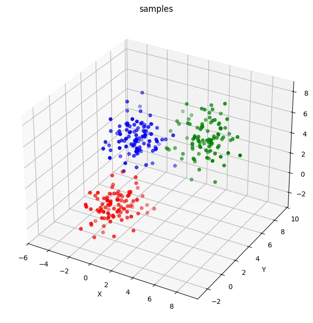
• 3つのグループが存在しており、それぞれがある程度固まっている状態になっている。

SNEをフィッティングする

X = datas
Y = fit_sne(X, n_components=2, perplexity=10.0, learning_rate=0.1, n_iter=1000)

• そこそこ時間がかかるので、気長に待ちましょう

2次元で可視化してみる。

# 可視化
fig = plt.figure(figsize=(8, 8))
ax = fig.add_subplot()

for i in range(n_clusters):
    cluster_datas = Y[labels == i]
    ax.scatter(cluster_datas[:, 0],
               cluster_datas[:, 1],
               marker='o',
               color=colours[i])

# タイトル
ax.set_title('samples')

# グラフを表示
plt.show()

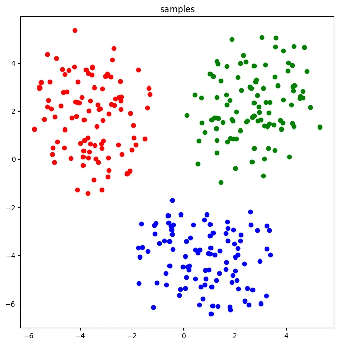
• ちゃんと3つのグループがそれぞれわかれるように低次元圧縮できた。

まとめ

• SNEをライブラリを使わずにスクラッチで実装した。
• 更新式は実装の簡易性を優先して、正しいものではないが、ちゃんと収束して、高次元空間のデータを低次元空間に圧縮することができた