お久しぶりの投稿です。
本日のテーマ
過去に書いた自分の記事に突っ込みを入れます。
過去に、lmer/glmerで信頼区間を算出する方法、としてconfint.mermod関数を紹介しました。
https://qiita.com/Jwellyfish/items/4b667a4dd1e0da18ee9f
現時点では (おそらくその当時も) もっと簡単な方法が存在していますので、そのご紹介です。
併せて、効果量 (effect size/risk ratio) と信頼区間をプロットする方法も紹介します。
データはHSAURパッケージのBtheBを使うことにします。
概要
lmer()/glmer()で作成されたmerModオブジェクトにbroom::tidy()を噛ませることで、tibbleとして出力してくれます。summary(lmer/glmer) ではp値および信頼区間を算出してくれませんが、broom::tidy()の引数conf.int = TRUEを設定することで信頼区間を出力してくれます。broom::tidy()で出力した効果量と信頼区間をforestplot::forestplot()に引き渡すことで、簡単に効果量をプロットできます。
準備
まずはBtheBを準備しましょう。
この辺の前処理は、REQUIER02の土屋さんのご発表をtidyverseで再現したものです。
> library(HSAUR)
> data <- BtheB %>%
  tibble::rownames_to_column(var = "ID") # adding rownames as a variable "ID"

> head(data)
  ID drug length treatment bdi.pre bdi.2m bdi.4m bdi.6m bdi.8m
1  1   No    >6m       TAU      29      2      2     NA     NA
2  2  Yes    >6m     BtheB      32     16     24     17     20
3  3  Yes    <6m       TAU      25     20     NA     NA     NA
4  4   No    >6m     BtheB      21     17     16     10      9
5  5  Yes    >6m     BtheB      26     23     NA     NA     NA
6  6  Yes    <6m     BtheB       7      0      0      0      0
BtheBデータは横持ちなので、縦持ちに変換します。
data1 <- data %>%
  gather(key = "month",
         value = "bdi",
         `bdi.2m`,`bdi.4m`,`bdi.6m`,`bdi.8m`
         )
横持時の変数名を時系列変数に変換します。
data1$month <- ifelse(data1$month == "bdi.2m", 2, data1$month)
data1$month <- ifelse(data1$month == "bdi.4m", 4, data1$month)
data1$month <- ifelse(data1$month == "bdi.6m", 6, data1$month)
data1$month <- ifelse(data1$month == "bdi.8m", 8, data1$month)

subset(data1, ID %in% c("1", "2", "3"))

> subset(data1, ID %in% c("1", "2", "3"))
    ID drug length treatment bdi.pre month bdi
1    1   No    >6m       TAU      29     2   2
2    2  Yes    >6m     BtheB      32     2  16
3    3  Yes    <6m       TAU      25     2  20
101  1   No    >6m       TAU      29     4   2
102  2  Yes    >6m     BtheB      32     4  24
103  3  Yes    <6m       TAU      25     4  NA
201  1   No    >6m       TAU      29     6  NA
202  2  Yes    >6m     BtheB      32     6  17
203  3  Yes    <6m       TAU      25     6  NA
301  1   No    >6m       TAU      29     8  NA
302  2  Yes    >6m     BtheB      32     8  20
303  3  Yes    <6m       TAU      25     8  NA
IDのrandom-slopeモデルでLMM (Linear Mixed Model)
> model01 <- lmer(bdi ~ treatment + month + bdi.pre + drug + length + (1|ID), data = data1)
> summary(model01)
Linear mixed model fit by REML ['lmerMod']
Formula: bdi ~ treatment + month + bdi.pre + drug + length + (1 | ID)
   Data: data1

REML criterion at convergence: 1859.8

Scaled residuals:
    Min      1Q  Median      3Q     Max
-2.7135 -0.4974 -0.0827  0.4084  3.7246

Random effects:
 Groups   Name        Variance Std.Dev.
 ID       (Intercept) 51.41    7.170
 Residual             25.52    5.052
Number of obs: 280, groups:  ID, 97

Fixed effects:
               Estimate Std. Error t value
(Intercept)     4.46830    2.26253   1.975
treatmentBtheB -2.35589    1.70968  -1.378
month4         -1.42557    0.81954  -1.739
month6         -2.64780    0.89391  -2.962
month8         -4.37403    0.92965  -4.705
bdi.pre         0.63909    0.07968   8.021
drugYes        -2.79416    1.76710  -1.581
length>6m       0.23614    1.67690   0.141

Correlation of Fixed Effects:
            (Intr) trtmBB month4 month6 month8 bdi.pr drugYs
tretmntBthB -0.395
month4      -0.141  0.021
month6      -0.138  0.025  0.440
month8      -0.125  0.019  0.423  0.432
bdi.pre     -0.691  0.122  0.012  0.025  0.018
drugYes     -0.076 -0.323 -0.016 -0.023 -0.023 -0.237
length>6m   -0.247  0.001 -0.034 -0.039 -0.039 -0.241  0.158
>
broom()を用いてtidyな感じで固定効果を抽出
> library(broom)
> es.model01 <- tidy(model01, effects = "fixed", conf.int = TRUE)
> es.model01
            term   estimate  std.error  statistic    conf.low  conf.high
1    (Intercept)  4.4683042 2.26253164  1.9749135  0.03382372  8.9027848
2 treatmentBtheB -2.3558889 1.70967729 -1.3779729 -5.70679483  0.9950170
3         month4 -1.4255691 0.81954421 -1.7394658 -3.03184629  0.1807080
4         month6 -2.6477953 0.89390922 -2.9620405 -4.39982513 -0.8957654
5         month8 -4.3740325 0.92964553 -4.7050541 -6.19610425 -2.5519607
6        bdi.pre  0.6390882 0.07967549  8.0211392  0.48292710  0.7952493
7        drugYes -2.7941559 1.76710183 -1.5812082 -6.25761183  0.6693001
8      length>6m  0.2361410 1.67689698  0.1408202 -3.05051673  3.5227986
>
大本のmodel01は線形混合モデルの結果です。
broom::tidy()を用いて綺麗にまとめたのがex.model01。引数conf.intをTRUEとすることで信頼区間を表示できます。信頼区間の水準はconf.levelで。effects = "fixed"を指定すると、固定効果のみを抽出できます。ランダム効果が効いてない場合にeffectsをデフォルト指定するとここでエラーを吐きます。
なお、glmer(family = binomial)、すなわちロジスティック回帰で一般化線形混合モデルを用いる場合、tidy関数のexponentiateは無効化されている模様 (glmではまだ有効?)。この辺、もう一工夫が必要そう。
broom()でまとめたlmer/glmerの結果をforestplotで出力
# plotting modeled effects
plot.es <- forestplot(
  labeltext = es.model01$term, mean = es.model01$estimate, lower = es.model01$conf.low, upper = es.model01$conf.high, # 変数名、効果量、信頼区間 (下限)、信頼区間 (上限)
  is.summary = FALSE, # メタアナっぽく表を同時表示するならTRUEに

  fn.ci_norm = fpDrawCircleCI, # マーカーの形状を指定
  boxsize = 0.3, # 主にマーカーの大きさを指定
  col = fpColors(box = "royalblue", lines = "gray", zero = "darkred"), # グラフ要素の色指定。
  colgap = unit(6, "mm"), # 変数間の間隔

  # grid = structure(c(-1, 1, 2, 3), gp = gpar(lty = 2, col = "#CCCCFF")), # グリッドの設定。お好みで。
  lineheight = unit(1, "cm"), # default: auto
  zero = 0, lwd.zero = 2, # X軸の0の設定。対数軸ならzero = 1、そうでなければzero = 0 (default)

  xtics = seq(from = -6, to = 9, by = 3), # X軸の軸ラベルの設定
  xlab = "BDI scores",
  txt_gp = fpTxtGp(label = gpar(fontfamily = "", cex = 1),
                   ticks = gpar(fontfamily = "", cex = 1),
                   xlab  = gpar(fontfamily = "", cex = 1)), # 文字のサイズ設定

  mar = unit(rep(5, times = 4), "mm") # グラフの四隅からのマージンの設定
)
ここでプロットされるグラフはggplot2系ではないので、jpeg()/png()とdev.off()で挟んであげましょう。
出力されたグラフがこちら。
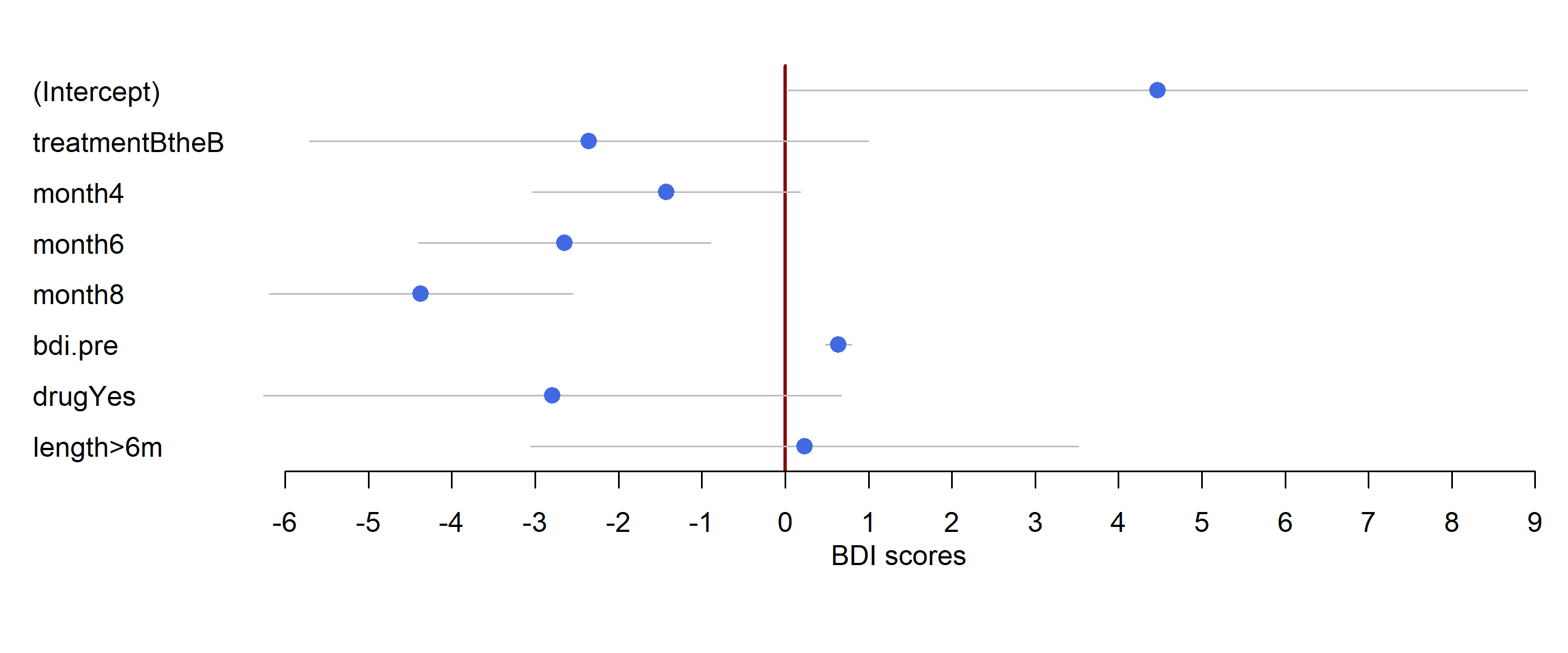
forestplot()のis.summary以降は描画の細かい設定で、効果量や信頼区間の限界値はlabeltextの行で指定済。推定結果をtibbleで返してくれるbroom::tidy()が活きてます。