State Space Models APIでonline forecast (refitもあるよ) 備忘録

概要

前回は状態空間モデルの仕組みが直感的に理解できる記述だったが、コードが長くなり仕組みに興味がない人には可読性が悪いのでここではstatsmodelsのAPIを使ってコーディングする。観測値を追加するたびにfitし直す（model.append(refit=True)）ことができるオプションもあるので計算コストと精度の変化も確認する。

• 実施期間: 2024年9月
• 環境：Ubuntu22.04LTS
• Python: condaのPython3.10

1. Dataset

データは前回と同じ東京における月毎の平均気温、気圧、湿度データを使用する。列名はそれぞれ['temperature', 'pressure', 'humidity']であり、内生変数が'temperature'、外生変数が'pressure'と'humidity'であることも同じ。

２. コード

下記コードのように状態方程式の変数とその共分散に関する操作は一切なく、statsmodelsがよろしく処理してくれる。状態を引き継ぐためのオーバラップも考慮する必要はない。ただし外生変数に関する注意事項は前回と同じ。

import time
import numpy as np
import pandas as pd
import statsmodels.api as sm
from statsmodels.tsa.statespace.sarimax import SARIMAX
import matplotlib.pyplot as plt
import sqlite3
from tqdm import tqdm
import pickle
import pmdarima as pm
from pmdarima import model_selection
import numpy as np
from matplotlib import pyplot as plt
from sklearn.metrics import root_mean_squared_error

def get_orders(endog_df, exdog_df, m=1, with_exog=False):
    if with_exog:
        auto_arima = pm.auto_arima(
                            y=endog_df, 
                            X=exdog_df, 
                            max_order = 5,      # p+q+P+Q
                            m = m,
                            seasonal=True, 
                            stepwise = True,
                            approximation = False,
                            information_criterion='aic',
                            error_action="ignore",
                            suppress_warnings=True)
    else:
        auto_arima = pm.auto_arima(
                            y=endog_df, 
                            max_order = 5,      # p+q+P+Q
                            m = m,
                            seasonal=True, 
                            stepwise = True,
                            approximation = False,
                            information_criterion='aic',
                            error_action="ignore",
                            suppress_warnings=True)
    # 実行
    return auto_arima


if __name__ == '__main__':
    df = pd.read_csv('tokyo_temp_monthly.csv')
    df['date'] = pd.to_datetime(df['date'], format='%Y/%m')
    df['date'] = pd.to_datetime(df['date']).dt.to_period('M').dt.to_timestamp()
    df = df.reset_index(drop=True).set_index('date')
    df = df.drop(columns='sunshine_hours')
    # df['pressure_rolling'] = df['pressure'].rolling(5).var()    #.shift(1)
    # df['humidity_rolling'] = df['humidity'].rolling(5).var()    #.shift(1)
    # df = df.dropna()
    df = df.asfreq('MS')

    with_exog = False
    initial_tw = 12 * 30
    m = 12       # the number of periods in each season

    # infer orders
    endog_data = df.iloc[:initial_tw]['temperature']
    exog_data = df.iloc[:initial_tw][['pressure', 'humidity']]
    auto_arima = get_orders(endog_data, exog_data, m, with_exog)
    with open('auto_arima.pickle', mode='wb') as fo:
        pickle.dump(auto_arima, fo)
    # with open('auto_arima.pickle', mode='br') as fi:
    #     auto_arima = pickle.load(fi)

    print(auto_arima.summary())

    kwargs = {'order': auto_arima.order, 
            #   'trend':'c', 
              'seasonal_order': auto_arima.seasonal_order, 
              'initialization': 'approximate_diffuse', 
              'enforce_stationarity': False, 
              'enforce_invertibility': False}

    if with_exog:
        model = SARIMAX(endog_data, exog=exog_data, **kwargs)
    else:
        model = SARIMAX(endog_data, **kwargs)
    model_fit = model.fit(disp=False)

    start = time.perf_counter()
    pred_tw = 1
    is_1st2 = True
    for t in tqdm(range(initial_tw, len(df)-pred_tw-1)):
        endog_data = df.iloc[t: t + pred_tw]['temperature']

        # forecast結果取得
        if with_exog:
            # prediction = filtered_results.get_forecast(steps=1, exog=df.iloc[t + pred_tw -1: t + pred_tw][['pressure_rolling', 'humidity_rolling']])
            exog_data = df.iloc[t: t + pred_tw][['pressure', 'humidity']]
            model_fit = model_fit.append(endog_data, exog=exog_data, refit=False)
            prediction = model_fit.get_forecast(
                steps=1, 
                exog=df.iloc[t+pred_tw: t+pred_tw+1][['pressure', 'humidity']]
                )
        else:
            model_fit = model_fit.append(endog_data, refit=True)
            prediction = model_fit.get_forecast(steps=1)

        if is_1st2:
            result_df = pd.concat([df.iloc[t+pred_tw: t+pred_tw+1]['temperature'], 
                                    prediction.predicted_mean, 
                                    prediction.conf_int(alpha=0.10)], axis=1)
            result_df = result_df.rename(columns={0: 'pred_mean'})
            is_1st2 = False
        else:
            wk_df = pd.concat([df.iloc[t+pred_tw: t+pred_tw+1]['temperature'], 
                                prediction.predicted_mean, 
                                prediction.conf_int(alpha=0.10)], axis=1)
            wk_df = wk_df.rename(columns={0: 'pred_mean'})
            result_df = pd.concat([result_df, wk_df])

    end = time.perf_counter()
    print('{:.2f}'.format((end-start)/60))
    
    result_df['base_line'] = result_df['temperature'].shift(1)
    result_df = result_df.dropna()
    result_df.to_csv('result_API_df_refit.csv')

    wk_result_lst = [[root_mean_squared_error(result_df['temperature'], result_df['base_line']), 
                        root_mean_squared_error(result_df['temperature'], result_df['pred_mean'])]]
    
    print(f'base_acc: {round(float(wk_result_lst[0][0]),5)}, acc: {round(float(wk_result_lst[0][1]),5)}')

2. 結果

下表の通り、1time step前の値を予測値とするbase lineと比べ、どれも格段に良い精度なことは明らか。
SSMの条件の違いについては外生変数がない方の精度が良くなっている。特にこの時の外生変数はカンニングしたものだったので、それで悪くなるとは思わなかった。気圧、湿度の変化が温度に寄与していないということ？もう少し内生変数と外生変数の勉強が必要。よくわからないのであれば外生変数は使用しないほうが良いだろう。
refitの有無については外生変数を使用しない場合でほぼ変化がない。計算コストが7.5倍もかかっているのであえてrefit=Trueを使用する必要はなさそう。
尚、下表にはないがrefit=Falseだと信頼区間幅は時間を追って変化なく、Trueにすることで変化が大きくなる。信頼区間を何らか使う予定があればrefitしても良いかも。

exog	refit	rmse	append time
なし	False	1.08465	10.80
なし	True	1.08970	75.26
あり	False	1.13206	13.02
あり	True	1.10771	75.43
base	base	4.13523	-

refit=Falseにした時の予測値と前回投稿の予測値がどの時点も全く同値だったことは確認済み。

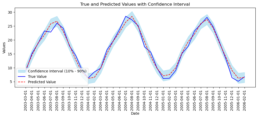
3. 結果描画

rmseが良かった時の３年分を描画する。他の条件も見た目はほぼ同じだった。

import pandas as pd
import matplotlib.pyplot as plt
import seaborn as sns

def draw_chart(df, month):
    # チャートのサイズを設定
    plt.figure(figsize=(12, 4))

    month = 36
    # 信頼区間を水色で満たす
    plt.fill_between(df.index[:month], df['lower temperature'].iloc[:month], df['upper temperature'].iloc[:month], color='skyblue', alpha=0.5, label='Confidence Interval (10% - 90%)')

    # "True" と "Pred" のラインをプロット
    sns.lineplot(x=df.index[:month], y=df['temperature'].iloc[:month], color='blue', label='True Value')
    sns.lineplot(x=df.index[:month], y=df['pred_mean'].iloc[:month], color='red', linestyle='--', label='Predicted Value')

    # ラベルとタイトルの設定
    plt.xlabel('Date')
    plt.ylabel('Values')
    plt.title('True and Predicted Values with Confidence Interval')
    plt.legend()

    plt.xticks(rotation=90)
    # プロットの表示
    plt.show()

df = pd.read_csv("result_API_df_refit_true_exog.csv", index_col=0)
draw_chart(df, 36)

以上