ReLU活性化関数

ReLU活性化関数

活性化関数にはシグモイド関数が伝統的に使われてきたが、最近ではReLU(Rectified Liner Unit)と呼ばれる活性化関数が人気である。2015年時点ではReLUが活性化関数として最善であるとまで言われていた。

ReLU

h(x) = x　(x > 0),　0　(0 \geqq x)

プログラム上の実装では...

def ReLU(0, x):
    return max(0, x)

シグモイド関数は入力のxがある程度大きくなると常に1に近い値を出力するので、入力の変化が出力に反映されにくくなります。その結果、誤差関数の重みパラメータに関する偏微分が0に近い値になり、勾配法による学習が遅くなるという問題は回避されます。また、プログラム上ではmax(0, x)として簡単に表すことができるので、計算が早いという利点もある。

ネットワークの中間層の活性化関数をReLUに変えて実行してみる。

import numpy as np
import matplotlib.pyplot as plt
import time

from keras.datasets import mnist
from keras.utils import to_categorical

from keras.models import Sequential
from keras.layers import Dense, Activation
from keras.optimizers import Adam

(x_train, y_train), (x_test, y_test) = mnist.load_data()

x_train = x_train.reshape(60000, 784)
x_train = x_train.astype('float32')
x_train = x_train / 255

num_classes = 10

y_train = to_categorical(y_train, num_classes)

x_test = x_test.reshape(10000, 784)
x_test = x_test.astype('float32')
x_test = x_test / 255

y_test = to_categorical(y_test, num_classes)

np.random.seed(1)

# Sequentialモデルの作成
model = Sequential()
model.add(Dense(16, input_dim=784, activation='relu'))
model.add(Dense(10, activation='softmax'))
model.compile(loss='categorical_crossentropy', optimizer=Adam(), metrics=['accuracy'])

# 学習
startTime = time.time()
history = model.fit(x_train, y_train, epochs=10, batch_size=1000, verbose=1, validation_data=(x_test, y_test))

# モデル評価
score = model.evaluate(x_test, y_test, verbose=0)
print('Test loss:', score[0])
print('Test accuracy:', score[1])

calculation_time = time.time() - startTime
print("Calculation time:{0:.3f} sec".format(calculation_time))

def show_prediction():
    n_show = 96
    y = model.predict(x_test)
    plt.figure(2, figsize=(12, 8))
    plt.gray()
    for i in range(n_show):
        plt.subplot(8, 12, i + 1)
        x = x_test[i, :]
        x = x.reshape(28, 28)
        plt.pcolor(1 - x)
        wk = y[i, :]
        prediction = np.argmax(wk)
        plt.text(22, 25.5, "%d" % prediction, fontsize=12)
        if prediction != np.argmax(y_test[i, :]):
            plt.plot([0, 27], [1, 1], color='cornflowerblue', linewidth=5)
        plt.xlim(0, 27)
        plt.ylim(27, 0)
        plt.xticks([], "")
        plt.yticks([], "")

show_prediction()
plt.show()

シグモイド関数使った場合では間違いが8個だったが、今回は4個まで減らすことができ、学習の精度が上がったと言える。

※シグモイド関数を使った実装は以下の記事にある。

このネットワークがどのようなパラメータを獲得していたのか、ネットワークモデルの中間層の重みパラメータを表示する。

import numpy as np
import matplotlib.pyplot as plt
import time

from keras.datasets import mnist
from keras.utils import to_categorical

from keras.models import Sequential
from keras.layers import Dense, Activation
from keras.optimizers import Adam

(x_train, y_train), (x_test, y_test) = mnist.load_data()

x_train = x_train.reshape(60000, 784)
x_train = x_train.astype('float32')
x_train = x_train / 255

num_classes = 10

y_train = to_categorical(y_train, num_classes)

x_test = x_test.reshape(10000, 784)
x_test = x_test.astype('float32')
x_test = x_test / 255

y_test = to_categorical(y_test, num_classes)

np.random.seed(1)

# Sequentialモデルの作成
model = Sequential()
model.add(Dense(16, input_dim=784, activation='relu'))
model.add(Dense(10, activation='softmax'))
model.compile(loss='categorical_crossentropy', optimizer=Adam(), metrics=['accuracy'])

# 学習
startTime = time.time()
history = model.fit(x_train, y_train, epochs=10, batch_size=1000, verbose=1, validation_data=(x_test, y_test))

# モデル評価
score = model.evaluate(x_test, y_test, verbose=0)
print('Test loss:', score[0])
print('Test accuracy:', score[1])

calculation_time = time.time() - startTime
print("Calculation time:{0:.3f} sec".format(calculation_time))

def show_prediction():
    n_show = 96
    y = model.predict(x_test)
    plt.figure(2, figsize=(12, 8))
    plt.gray()
    for i in range(n_show):
        plt.subplot(8, 12, i + 1)
        x = x_test[i, :]
        x = x.reshape(28, 28)
        plt.pcolor(1 - x)
        wk = y[i, :]
        prediction = np.argmax(wk)
        plt.text(22, 25.5, "%d" % prediction, fontsize=12)
        if prediction != np.argmax(y_test[i, :]):
            plt.plot([0, 27], [1, 1], color='cornflowerblue', linewidth=5)
        plt.xlim(0, 27)
        plt.ylim(27, 0)
        plt.xticks([], "")
        plt.yticks([], "")

w = model.layers[0].get_weights()[0]
plt.figure(1, figsize=(12, 3))
plt.gray()
plt.subplots_adjust(wspace=0.35, hspace=0.5)
for i in range(16):
    plt.subplot(2, 8, i + 1)
    w1 = w[:, i]
    w1 = w1.reshape(28, 28)
    plt.pcolor(-w1)
    plt.xlim(0, 27)
    plt.xlim(27, 0)
    plt.xticks([], "")
    plt.yticks([], "")
    plt.title("%d" % i)

plt.show()

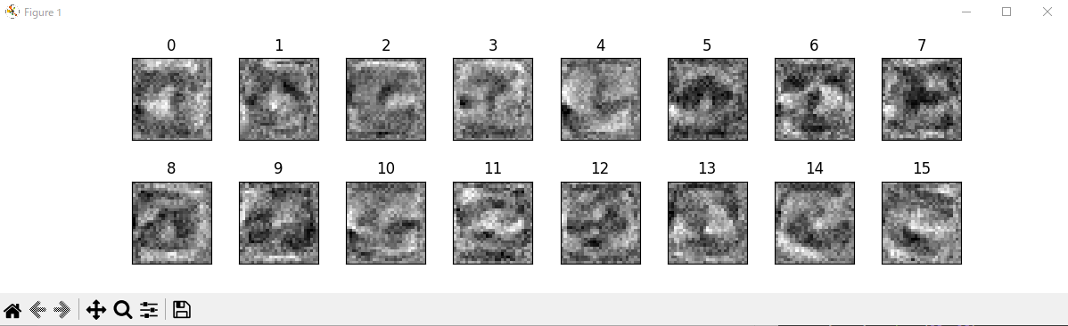
27×27の入力から中間層の16個のニューロンへの重みを図示している。重みの値が正の場合が黒、負の場合は白で表している。もともとは重みはランダムに設定されていいるが、この模様は学習によって獲得されたものになる。黒い部分に文字の一部があると、そのニューロンは活性死、白い部部に文字の一部があると、抑制される。