前回はグラフの基本を投稿しました。今回は様々な種類のグラフを作成し、投稿していきたいと思います。
散布図
from matplotlib import pyplot as plt
import numpy as np

# ランダムな点を生成する
x = np.random.rand(50)
y = np.random.rand(50)

# figureを生成する
fig = plt.figure()

# axをfigureに設定する
ax = fig.add_subplot(1, 1, 1)

# プロットマーカーの大きさ、色、透明度を変更
ax.scatter(x, y, s=300, alpha=0.5, linewidths=2, marker='*', c='#aaaaFF', edgecolors='blue')
plt.show()
実行結果

matplotlibで散布図を描画する場合、axes.scatterを使用します。引数でマーカーサイズ、色、形などを指定することが可能です。色は16進数カラーコード以外に、CSSのカラーネームを使用することもできます。また、利用できるマーカーの例として以下が挙げられます。
記号 マーカーの形
① ・ 点
② o 円
③ * 星印
④ + +
⑤ X ✕
⑥ D ひし形
棒グラフ
import matplotlib.pyplot as plt

# ラベル
label = ['A', 'B', 'C', 'D', 'E']

# 対象データ
x = [1, 2, 3, 4, 5]  # 横軸
height = [3, 5, 1, 2, 3]  # 値

# figureを生成する
fig = plt.figure()

# axをfigureに設定する
ax = fig.add_subplot(1, 1, 1)

# axesに棒グラフを設定する
ax.bar(x, height, label=label, linewidth=1, edgecolor="#000000")
# 表示する
plt.show()
実行結果
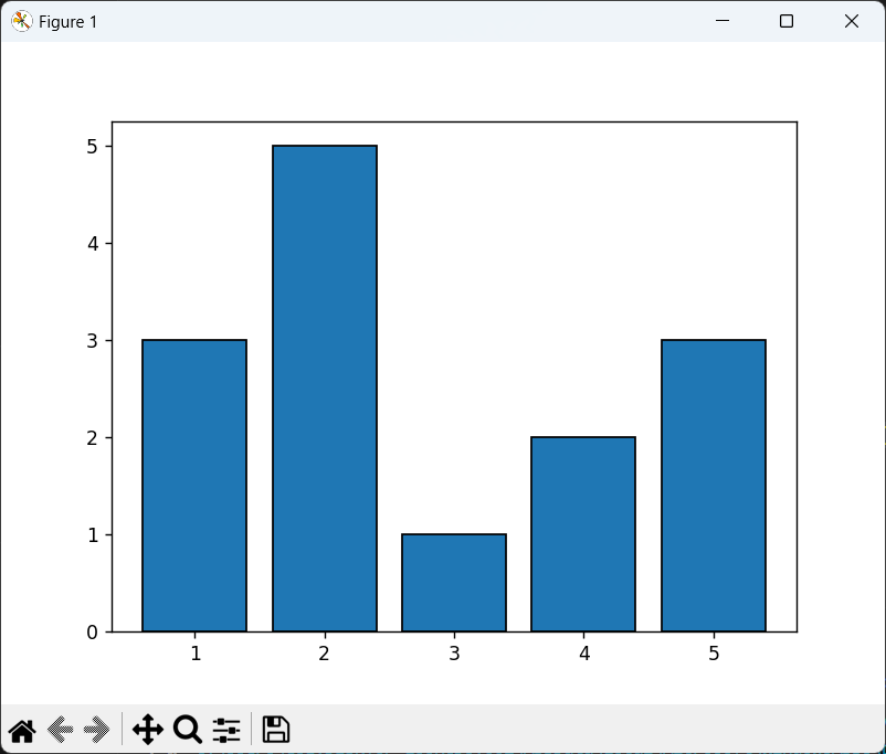
matplotlibで棒グラフを作成する場合、axes.barを使用します。引数で幅、ラベル、色などを指定することが可能です。上記のコードでは、A 〜 Eの各値に対して棒グラフを描画しています。また、linewidth、edgecolorでグラフの枠線の太さと色を指定しています。
折れ線グラフ
import matplotlib.pyplot as plt

# 対象データ
x = [1, 2, 3, 4, 5]

y1 = [100, 300, 200, 500, 0]
y2 = [150, 350, 250, 550, 50]
y3 = [200, 400, 300, 600, 100]
y4 = [250, 450, 350, 650, 150]

# figureを生成する
fig = plt.figure()

# axをfigureに設定する
ax = fig.add_subplot(1, 1, 1)

# axesにplot
ax.plot(x, y1, "-", c="#ff0000", linewidth=1, marker='*', alpha=1)
ax.plot(x, y2, "--", c="#00ff00", linewidth=2, marker='o', alpha=0.5)
ax.plot(x, y3, "-.", c="#0000ff", linewidth=4, marker='D', alpha=0.5)
ax.plot(x, y4, ":", c="#ff00ff", linewidth=4, marker='x', alpha=0.5)

# 表示する
plt.show()
実行結果
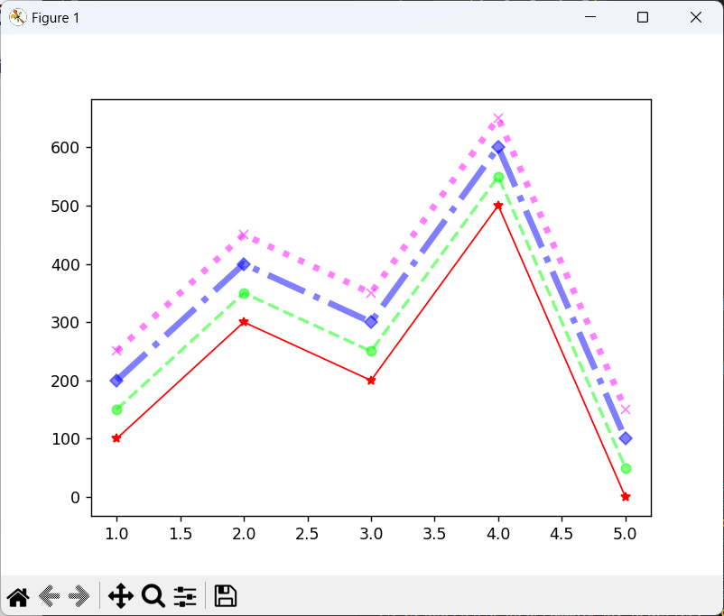
matplotlibで折れ線グラフを描画する場合、axes.plotを使用します。引数で折れ線の種類、色、太さ、マーカーの種類などを指定することができます。線の種類は、以下を指定することができます。
記号 意味
① - 実線
② -- 破線
③ -. 点+破線
④ : 点線
関数のグラフ
import matplotlib.pyplot as plt
import numpy as np

# 対象データ
x = np.linspace(0, 5, 100)  # x軸の値
y1 = x ** 2
y2 = np.sin(x)

# figureを生成する
fig = plt.figure()

# axをfigureに設定する
ax = fig.add_subplot(1, 1, 1)

# axesにplot
ax.plot(x, y1, "-")
ax.plot(x, y2, "-")

# 表示する
plt.show()
実行結果

NumPyのlinspaceを使用すると、指定区間内で、十分に要素数が多い関数のndarrayを作成することができます。また、ndarrayはユニバーサル関数で要素全体に関数を作用させることができるため、ax.plotと併せて使用すると滑らかなグラフを描画することができます。上記のコードでは、閉区間[0.5]を100で分割した、区間ごとの三角関数と二次関数のグラフを描画しています。
円グラフ
import matplotlib.pyplot as pltの

# 対象データ
label = ["A", "B", "C", "D", "E"]
x = [40, 30, 15, 10, 5]

# figureを生成する
fig = plt.figure()

# axをfigureに設定する
ax = fig.add_subplot(1, 1, 1)

# axesにplot
ax.pie(x, labels=label, counterclock=False, startangle=90)

# 表示補正
ax.axis('equal')

# 表示する
plt.show()
実行結果

matplotlibで円グラフを 描画する場合、axes.pieを使用します。引数で線の種類、色、太さ、マーカーの種類などを指定することが可能です。デフォルトパラメータが少し特殊で、パラメータを指定しない場合、円グラフの開始が3時の方向から、反時計回りで描画されます。このため、12時の方向から時計回りにしたい場合、counterclockとstartangleの指定が必要です。また、環境次第で円が押しつぶされるため、ax.axis(equal)を指定します。上記のコードでは、A〜Eのデータの円グラフを描画しています。
ヒストグラム
import matplotlib.pyplot as plt
import numpy as np

# 対象データ
x = np.random.normal(0, 10, 1000)
# figureを生成する
fig = plt.figure()

# axをfigureに設定する
ax = fig.add_subplot(1, 1, 1)

# axesにplot
ax.hist(x, bins=10, color="#00AAFF", ec="#0000FF", alpha=0.5)

# 表示する
plt.show()
実行結果

matplotlibでヒストグラムを描画する場合、axes.histを使用します。パラメータを階級数や色を指定することが可能です。引数binsは少し変わった引数で、引数の型が何種類かあります。整数を指定するとその数の分の区間に分割します。一方で配列を指定するとその配列の階級となります。また、後述のスタージェスの公式で自動的に階級分けすることもできます。上記のコードでは、要素数1000個、平均0、標準格差10の正規分布の乱数の配列を生成し、ヒストグラムで可視化しています。
以上となります。前回今回含め、非常に中身の濃い内容でした。引き続き学習し投稿していきたいと思います。
エンジニアファーストの会社 株式会社CRE-COエンジニアリングサービス
H.M