MeanF1Scoreについて実験してみた

この記事を書くに至った経緯

現在SIGNATEで開催されている第2回金融データ活用チャレンジにて、MeanF1Score（MacroF1Score）が評価関数として採用されており、私自身この評価関数を扱ったコンペに参加したことがなく、とりあえず「正例と負例は与えられたトレーニングデータと同じ数にしておけばいんだよね。」と軽く考えていました。コンペが進むに従って、どうやらデータよりやや負例を少なくした方が、良いスコアが出るようになり、参加者のslackでも同様のことを提唱されている方がいました。負例をトレーニングと同じ数にしなくていいのか？について、シミュレーションも含めて検証してみました。

下準備

最低限の下処理をして、5分割のクロスバリデーションにより、lightGBMでトレーニングを行い、予測済みのバリデーションデータを得ます。「クロスバリデーションとは？」という方は、この辺りを参照してください。交差検証（Python実装）を徹底解説！図解・サンプル実装コードあり

前処理

# 必要なライブラリをインポート
import numpy as np
import pandas as pd
import matplotlib.pyplot as plt
import seaborn as sns
import lightgbm as lgb
from dateutil.relativedelta import relativedelta
import copy
from scipy.stats import hmean
import random

from sklearn.model_selection import StratifiedKFold
from sklearn.model_selection import train_test_split
from sklearn.metrics import f1_score
from sklearn.metrics import log_loss
from sklearn.metrics import precision_recall_curve
from sklearn.metrics import mean_squared_error

pd.set_option('display.max_columns', 2000)
pd.set_option('display.max_rows', 2000)
pd.set_option('display.max_colwidth',100000)
pd.set_option('display.width', 10000)
%matplotlib inline


# 前処理
def data_pre(df):
    df[['DisbursementGross',  'GrAppv', 'SBA_Appv']]= \
    df[['DisbursementGross',  'GrAppv', 'SBA_Appv']].applymap(lambda x: x.strip().replace('$', '').replace(',', ''))

    #object→float
    for col in ['DisbursementGross',  'GrAppv', 'SBA_Appv'
               ]:
        df[col] = df[col].astype(float)

    #object→category
    for  col in df.columns:
        if df[col].dtype=='object':
            df[col]  = df[col].astype("category")
    return df

# 前処理の内容を適用（df=がトレーニングデータ、test_dfがテストデータ） 
df=data_pre(df)
test_df=data_pre(test_df)

最低限、データ型だけ、lightGBMが適用できるように変更します。

モデル作成

# モデル作成 lgb
def model_lgb_kf(df):

    k=5
    models = []
    valid_scores = []
    skf = StratifiedKFold(n_splits=k, shuffle=True, random_state=0)


    col = 'MIS_Status'
    y = df[col]
    X = df.drop(col,axis=1)
    predicted = copy.copy(df[col])

    # kfoldで分割
    for train_index, test_index in skf.split(X, y):

        X_train = X.iloc[train_index]
        y_train = y.iloc[train_index]
        X_test = X.iloc[test_index]
        y_test = y.iloc[test_index]

        # データセットを生成する
        lgb_train = lgb.Dataset(X_train, y_train)

        # モデル評価用
        lgb_valid = lgb.Dataset(X_test,y_test)

        params =  {'objective': 'binary',
                    'metric': "binary_logloss",
                    'learning_rate': 0.01,
                    'feature_fraction': 0.30,
                    'max_depth': 6,
                    'early_stopping_round': 50,
                    'num_iterations': 1000}

        model = lgb.train(params
                          ,lgb_train
                          ,valid_sets=lgb_valid
                        ,callbacks=[
                lgb.early_stopping(stopping_rounds=50, verbose=True),
                lgb.log_evaluation(100),
            ]
                          )

        models.append(model)
        pred =model.predict(X_test)
        predicted.iloc[test_index]=pred

    return models,predicted

models_lgb,predicted_lgb=model_lgb_kf(df)

# 作成した予測値を貼り付け
df['predicted_lgb']=predicted_lgb

パラメータ等は適当です。ひとまずこれで、トレーニンングデータの予測値が完成しました。（ちなみにこれだけでも閾値を調節すれば、リーダーボードで0.686(2/2現在ブロンズライン付近）あたりになります。）

本題

まず、今回予想したものに対して最適な閾値を測ります。自分でいちから実装するのは、骨が折れるので便利な道具(sklearn.metrics.precision_recall_curve)に頼ります。
使い方はこの記事を参考にしました。
F値とPrecisionとRecallのトレードオフを理解する(超重要!!)【機械学習入門21】

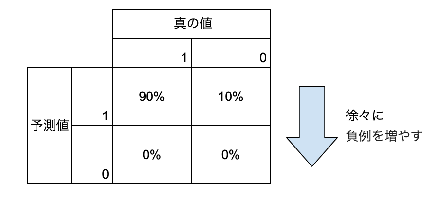
今回で言うと正例（ターゲット=1)と負例の比が9:1程度なので、最初全て正例と予想して、徐々に負例の予想の数を増やした時に、MeanF1Scoreがどう動くか考えると、見通しがいいと思ったのでその方向で作成しています。すなわち以下の図のような考え方です。

正例側のprecision_recall_curve

# 正例
precision_1, recall_1, thresholds = precision_recall_curve(df['MIS_Status'], df['predicted_lgb'])
# 描画
ax = plt.subplot()
ax.invert_xaxis()
plt.plot(recall_1,precision_1)
plt.xlabel('Recall')
plt.ylabel('Precision')
plt.title('Precision Recall Curve')

plt.show()

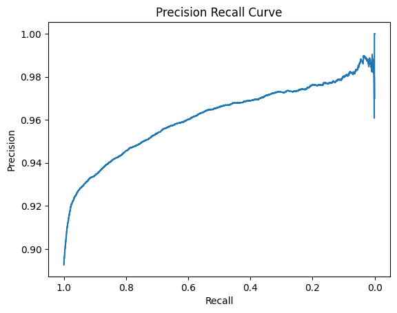
全て正例と予想すると、Recall=1.0,Rrecision=正例のデータ数/データ数≒0.9
となるので問題なさそうですね。最初は負例を精度効率よく見つけられるのでRrecisionが上がりやすいですが、徐々に精度が落ちてくるのでPrecisionの伸びが緩やかになっていくと言うのも実感に合っています。

負例側のprecision_recall_curve

precision_0, recall_0, thresholds = precision_recall_curve(1-df['MIS_Status'], 1-df['predicted_lgb'])

# 描画
plt.plot(recall_0,precision_0)
plt.xlabel('Recall')
plt.ylabel('Precision')
plt.title('Precision Recall Curve')
plt.show()

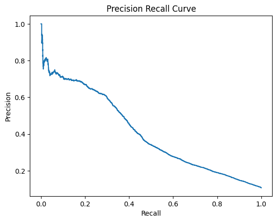
負例側から考えると、最初は効率よく負例を見つけられるのでPrecisionが高い値になりますが、徐々に精度が下がってくるので、Precisionが低くなっていき、最終的に全て負例とした時、負例のデータ数/データ数≒0.1に落ちつきます。

MeanF1Score

# 逆転しておく
recall_0=recall_0[::-1]
precision_0=precision_0[::-1]

# F値計算
mean_f1_scores = []
f1_scores_1 = []
f1_scores_0 = []
for p_0, r_0 , p_1 , r_1 in zip(precision_0, recall_0,precision_1, recall_1):
    f1_0 = hmean([p_0, r_0])
    f1_1 = hmean([p_1, r_1])
    mean_f1=(f1_0+f1_1)/2
    mean_f1_scores.append(mean_f1)
    f1_scores_0.append(f1_0)
    f1_scores_1.append(f1_1)
# F値を描画
plt.plot(mean_f1_scores[:-1], label='mean_f1 score')
plt.plot(f1_scores_1[:-1], label='f1 score_1')
plt.plot(f1_scores_0[:-1], label='f1 score_0')

plt.xlabel('threshold')
plt.legend()

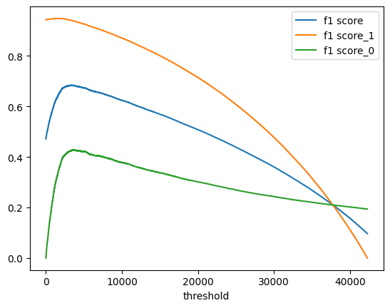
最初全て正例と予想し、徐々に負例を多くしていく形でのF1_Score が描画できました。最初は負例側のF1Scoreが急激に伸びますが、徐々に頭打ちになる様子がわかります。mean_F1Scoreが最高値をとる場所を調べると、

print(f'{np.argmax(mean_f1_scores)}th is highest f1 score ={np.max(mean_f1_scores):.5f}')

3450th is highest f1 score =0.68406

実際の負例の件数（4540件）よりかなり少なめの場所でピークをとっています。
ここについてもう少し掘り下げるため、以下のような設定でmeanF1スコアがどうなるか検証してみます。

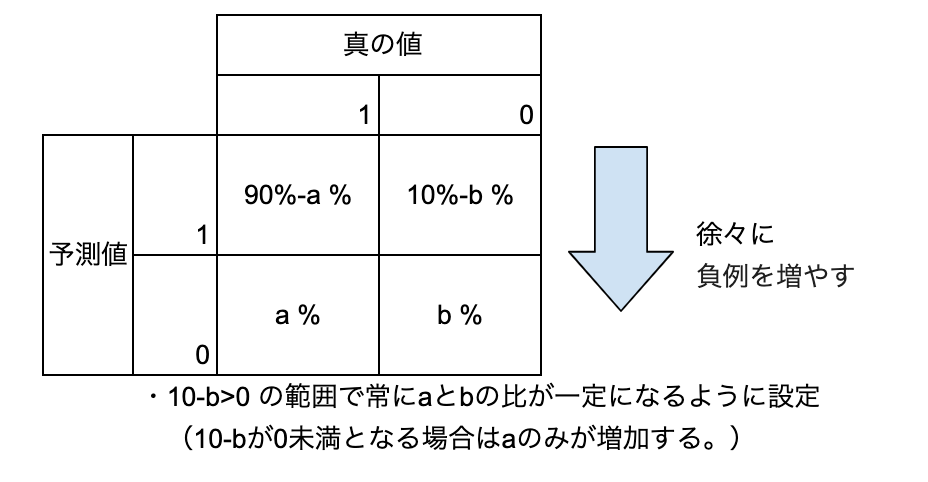
通常最初の方が、予測精度が高いのでだんだんbに対してaが大きくなっていきますが、あえて精度が変わらないモデルの場合はmeanF1Scoreがどんな値を取るかみてみます。

a:b=1:1の場合

なぜか同じ予測値を割り当てるとうまくいかなかったので、目的の予測値の付近に乱数を発生させてみました。

df['predict_50%']=0
df['predict_50%']=df['predict_50%'].apply( lambda x: np.random.random() )/10+0.45

# ランダムサンプルの抽出
df['predict_50%'].loc[random.sample(list(df[df['MIS_Status']==1].index),33227)]=df['predict_50%'].apply( lambda x: np.random.random() )/10+0.9
df=df.sample(frac=1)

a:b=1:1なので、負例と正例が同数となるように0.5付近の乱数を設定し、残りは、0.9付近の乱数を設定しておきました。

df['predict_50%'].value_counts().head(10)

0.997727 1
0.959753 1
0.990291 1
0.988685 1
0.964150 1
0.945119 1
0.997668 1
0.973218 1
0.512906 1
0.932513 1
Name: predict_50%, dtype: int64

問題なさそうです。MeanF1Scoreを出力します。

precision_1_50, recall_1_50, thresholds = precision_recall_curve(df['MIS_Status'], df['predict_50%'])
precision_0_50, recall_0_50, thresholds = precision_recall_curve(1-df['MIS_Status'], 1-df['predict_50%'])

# 逆転しておく
recall_0_50=recall_0_50[::-1]
precision_0_50=precision_0_50[::-1]

# F値計算
mean_f1_scores_50 = []
f1_scores_1_50 = []
f1_scores_0_50 = []
for p_0, r_0 , p_1 , r_1 in zip(precision_0_50, recall_0_50,precision_1_50, recall_1_50):
    f1_0 = hmean([p_0, r_0])
    f1_1 = hmean([p_1, r_1])
    mean_f1=(f1_0+f1_1)/2
    mean_f1_scores_50.append(mean_f1)
    f1_scores_0_50.append(f1_0)
    f1_scores_1_50.append(f1_1)
# Precision, Recall, F値を描画
plt.plot(mean_f1_scores_50[:-1], label='mean_f1_scores_50')
plt.plot(f1_scores_1_50[:-1], label='f1_scores_1_50')
plt.plot(f1_scores_0_50[:-1], label='f1_scores_0_50')

plt.xlabel('threshold')
plt.legend()

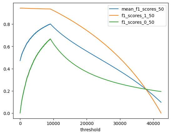
print(f'{np.argmax(mean_f1_scores_50)}th is highest f1 score ={np.max(mean_f1_scores_50):.5f}')

9079th is highest f1 score =0.80139

負例がなくなるところ（4540*2）までmeanF1Scoreが上昇しているのがわかります。今回のLightGBMの予想と比較すると、

# Precision, Recall, F値を描画(vs 閾値)
plt.figure(figsize=(8 ,6))
plt.plot(mean_f1_scores[:-1], label='mean_f1_score')
plt.plot(mean_f1_scores_50[:-1], label='mean_f1_scores_50')


plt.plot(recall_0,precision_0)
plt.ylim(0.4, 0.9)
plt.xlim(0, 10000)

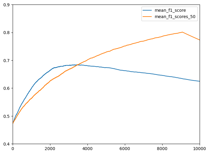
最初は、lightGBM予想の方が上にきてきますが、3500のあたりで抜かれていることがわかります。今回の設定だと、a+bの合計（負例と予想する件数）が同じ場合、a:bでMeanF1Scoreが決定されるため、このあたりでLightGBMの予想もa:b=1:1となっているのだと思います。察するに今回のデータは、少数の案件を高精度で予測できる特徴量がいくつかあるので、それが尽きるまでは高精度で予測できるが、それを使い果たすと精度が急激に低下するのだと思いました。特徴量の作り込みによって、3000~5000番目あたりの予測精度を上げ、予測精度の低下が緩やかになれば、山のピークは右側に移動するのではないかと思います。逆に0~2000番目の精度が上昇して、予想精度の低下が急になれば、ピークが左側に移動すると思います。

終わりに

実験する前は、「正例と負例の割合はとりあえずデータと同じにしておけばいいでしょ」と思っていましたが、精度低下が緩やかなモデルは、ピークが遅く、逆に最初の精度はいいが低下が激しいモデルはピークが早いことがわかりました。何事も実験してみるものですね。