PythonとGridDBによるフェイクニュースの検出 #Python

このような記事を目にするたびに、私たちは本能的に「何かおかしい」と感じるのです。あまりに多くの記事があるため、正しいものと間違ったものを選別するのは不可能に近いでしょう。

フェイクニュースは、2つの方法で主張することができます。第1に、事実に対する反論。2つ目は、使用されている言語です。前者は、自動クエリシステムとインターネットへの実質的な検索によってのみ達成可能です。後者は、自然言語処理パイプラインとそれに続く機械学習パイプラインによって可能となります。

この記事の目的は、フェイクまたはリアルとラベル付けされたニュースデータをモデル化することです。GridDBを使用してデータを抽出し、次に前処理のステップを実行し、最後に機械学習モデルを構築しましょう。

チュートリアルの概要は以下の通りです。

データセット概要
必要なライブラリのインポート
データセットの読み込み
データのクリーニングと前処理
機械学習モデルの構築
モデルの評価
まとめ

前提条件と環境設定

このチュートリアルは、Windows オペレーティングシステム上の Anaconda Navigator (Python バージョン - 3.8.3) で実行されます。チュートリアルを続ける前に、以下のパッケージがインストールされている必要があります。

Pandas
NumPy
Scikit-learn
Matplotlib
Seaborn
Tensorflow
Keras
nltk
re
patoolib
urllib
griddb_python

これらのパッケージは Conda の仮想環境に conda install package-name を使ってインストールすることができます。ターミナルやコマンドプロンプトから直接Pythonを使っている場合は、 pip install package-name でインストールできます。

GridDBのインストール

このチュートリアルでは、データセットをロードする際に、GridDB を使用する方法と、Pandas を使用する方法の 2 種類を取り上げます。Pythonを使用してGridDBにアクセスするためには、以下のパッケージも予めインストールしておく必要があります。

GridDB Cクライアント
SWIG (Simplified Wrapper and Interface Generator)
GridDB Pythonクライアント

1. データセット概要

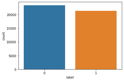
データセットは、偽物と本物のニュースが同数程度含まれる約40000記事から構成されます。ほとんどのニュースは米国の新聞から収集され、米国の政治、世界ニュース、ニュースなどが含まれています。

https://www.kaggle.com/datasets/clmentbisaillon/fake-and-real-news-dataset

2. 必要なライブラリのインポート

#import griddb_python as griddb

import numpy as np
import pandas as pd
import matplotlib.pyplot as plt
import seaborn as sns

import urllib.request
import patoolib

import nltk
import string
from nltk.corpus import stopwords
import re

import tensorflow as tf
from keras.preprocessing.text import Tokenizer
from tensorflow.keras.utils import to_categorical
from keras.preprocessing.sequence import pad_sequences

from sklearn.metrics import classification_report,confusion_matrix,accuracy_score
from sklearn.model_selection import train_test_split

import warnings
warnings.filterwarnings('ignore')
%matplotlib inline

3. データセットの読み込み

続けて、データセットをノートブックにロードしてみましょう。

3.a GridDBを利用する

GridDBは、IoTやビッグデータに最適な高スケーラブルNoSQLデータベースです。GridDBの理念の根幹は、IoTに最適化された汎用性の高いデータストアの提供、高い拡張性の提供、高性能なチューニング、高い信頼性の確保にあります。

大量のデータを保存する場合、CSVファイルでは面倒なことがあります。GridDBは、オープンソースで拡張性の高いデータベースであるため、完璧な代替手段として機能します。GridDBは、スケーラブルなインメモリ型NoSQLデータベースで、大量のデータを簡単に保存することができます。GridDBを初めて使う場合は、GridDBへの読み書みのチュートリアルが役に立ちます。

すでにデータベースのセットアップが完了していると仮定して、今度はデータセットをロードするためのSQLクエリをpythonで書いてみましょう。

factory = griddb.StoreFactory.get_instance()

# Initialize the GridDB container (enter your database credentials)
try:
    gridstore = factory.get_store(host=host_name, port=your_port, 
            cluster_name=cluster_name, username=admin, 
            password=admin)

    info = griddb.ContainerInfo("false_news",
                    [["title", griddb.Type.STRING],["text", griddb.Type.STRING],["subject", griddb.Type.STRING],
                     ["date", griddb.Type.TIMESTAMP],
                    griddb.ContainerType.COLLECTION, True)
    cont = gridstore.put_container(info) 
    data = pd.read_csv("False.csv")
    #Add data
    for i in range(len(data)):
        ret = cont.put(data.iloc[i, :])
    print("Data added successfully")
                     
try:
    gridstore = factory.get_store(host=host_name, port=your_port, 
            cluster_name=cluster_name, username=admin, 
            password=admin)

    info = griddb.ContainerInfo("true_news",
                    [["title", griddb.Type.STRING],["text", griddb.Type.STRING],["subject", griddb.Type.STRING],
                     ["date", griddb.Type.TIMESTAMP],
                    griddb.ContainerType.COLLECTION, True)
    cont = gridstore.put_container(info) 
    data = pd.read_csv("True.csv")
    #Add data
    for i in range(len(data)):
        ret = cont.put(data.iloc[i, :])
    print("Data added successfully")

pandasライブラリが提供するread_sql_query関数は、取得したデータをパンダのデータフレームに変換し、ユーザーが作業しやすいようにします。

sql_statement1 = ('SELECT * FROM false_news')
false = pd.read_sql_query(sql_statement, cont)

sql_statement2 = ('SELECT * FROM true_news')
true = pd.read_sql_query(sql_statement, cont)

変数 cont には、データが格納されているコンテナ情報が格納されていることに注意してください。credit_card_dataset をコンテナの名前に置き換えてください。詳細は、チュートリアルGridDBへの読み書みを参照してください。

IoTやビッグデータのユースケースに関して言えば、GridDBはリレーショナルやNoSQLの領域の他のデータベースの中で明らかに際立っています。全体として、GridDBは高可用性とデータ保持を必要とするミッションクリティカルなアプリケーションのために、複数の信頼性機能を提供しています。

3.b pandasのread_csvを使用する

また、Pandasの read_csv 関数を使用してデータを読み込むこともできます。どちらの方法を使っても、データはpandasのdataframeの形で読み込まれるので、上記のどちらの方法も同じ出力になります。

true = pd.read_csv("True.csv")
false = pd.read_csv("Fake.csv")

4. データクリーニングと前処理

true['label'] = 1
false['label'] = 0

2つのデータセットを1つにまとめ、テキストとタイトルを1つのカラムに追加します。

news = pd.concat([true,false]) 
news['text'] = news['text'] + " " + news['title']
df=news.drop(["date","title","subject"],axis=1)

sns.countplot(x="label", data=news);
plt.show()

df.head()

	text	label
0	WASHINGTON (Reuters) - The head of a conservat...	1
1	WASHINGTON (Reuters) - Transgender people will...	1
2	WASHINGTON (Reuters) - The special counsel inv...	1
3	WASHINGTON (Reuters) - Trump campaign adviser ...	1
4	SEATTLE/WASHINGTON (Reuters) - President Donal...	1

生のメッセージ（文字の列）をベクトル（数字の列）に変換する必要があります。その前に、句読点を削除、数字を削除、タグの削除、URLの削除、ストップワードの削除、ニュースの小文字への変更、Lemmatisationといったことを行う必要があります。

以下の4つの関数は、句読点(<,.': など)、数字、タグ、URLの削除に役立ちます。

def rem_punctuation(text):
  return text.translate(str.maketrans('','',string.punctuation))

def rem_numbers(text):
  return re.sub('[0-9]+','',text)


def rem_urls(text):
  return re.sub('https?:\S+','',text)


def rem_tags(text):
  return re.sub('&lt;.*?>'," ",text)

df['text'].apply(rem_urls)
df['text'].apply(rem_punctuation)
df['text'].apply(rem_tags)
df['text'].apply(rem_numbers)

0        WASHINGTON (Reuters) - The head of a conservat...
1        WASHINGTON (Reuters) - Transgender people will...
2        WASHINGTON (Reuters) - The special counsel inv...
3        WASHINGTON (Reuters) - Trump campaign adviser ...
4        SEATTLE/WASHINGTON (Reuters) - President Donal...
                               ...                        
23476    st Century Wire says As WIRE reported earlier ...
23477    st Century Wire says It s a familiar theme. Wh...
23478    Patrick Henningsen  st Century WireRemember wh...
23479    st Century Wire says Al Jazeera America will g...
23480    st Century Wire says As WIRE predicted in its ...
Name: text, Length: 44898, dtype: object

rem_stopwords() は、ストップワードを削除し、単語を小文字に変換する関数です。

stop = set(stopwords.words('english'))

def rem_stopwords(df_news):
    
    words = [ch for ch in df_news if ch not in stop]
    words= "".join(words).split()
    words= [words.lower() for words in df_news.split()]
    
    return words   

df['text'].apply(rem_stopwords)

0        [washington, (reuters), -, the, head, of, a, c...
1        [washington, (reuters), -, transgender, people...
2        [washington, (reuters), -, the, special, couns...
3        [washington, (reuters), -, trump, campaign, ad...
4        [seattle/washington, (reuters), -, president, ...
                               ...                        
23476    [21st, century, wire, says, as, 21wire, report...
23477    [21st, century, wire, says, it, s, a, familiar...
23478    [patrick, henningsen, 21st, century, wireremem...
23479    [21st, century, wire, says, al, jazeera, ameri...
23480    [21st, century, wire, says, as, 21wire, predic...
Name: text, Length: 44898, dtype: object

Lemmatizationは、単語の語彙と形態素解析を行い、通常、屈折語尾のみを除去することを目的としています。

from nltk.stem import WordNetLemmatizer
#nltk.download('wordnet')
lemmatizer = WordNetLemmatizer()

def lemmatize_words(text):
  lemmas = []
  for word in text.split():
    lemmas.append(lemmatizer.lemmatize(word))
  return " ".join(lemmas)

df['text'].apply(lemmatize_words)

0        WASHINGTON (Reuters) - The head of a conservat...
1        WASHINGTON (Reuters) - Transgender people will...
2        WASHINGTON (Reuters) - The special counsel inv...
3        WASHINGTON (Reuters) - Trump campaign adviser ...
4        SEATTLE/WASHINGTON (Reuters) - President Donal...
                               ...                        
23476    21st Century Wire say As 21WIRE reported earli...
23477    21st Century Wire say It s a familiar theme. W...
23478    Patrick Henningsen 21st Century WireRemember w...
23479    21st Century Wire say Al Jazeera America will ...
23480    21st Century Wire say As 21WIRE predicted in i...
Name: text, Length: 44898, dtype: object

トークン化・パディング

トークン化とは、テキストを単語に分解する処理のことです。トークン化はどの文字でも行うことができますが、最も一般的な方法はスペース文字で行う方法です。

当然ながら、文の中には長いものや短いものがあります。そこで、入力の大きさを揃えるために、パディングを用います。

x = df['text'].values
y= df['label'].values

tokenizer = Tokenizer()
tokenizer.fit_on_texts(x)
word_to_index = tokenizer.word_index
x = tokenizer.texts_to_sequences(x)

すべてのニュースを250字以内に収め、250字未満のニュースにはパディングを追加し、長いものは切り捨てることができます。

vocab_size =  len(word_to_index)
oov_tok = "<oov>"
max_length = 250
embedding_dim = 100

x = pad_sequences(x, maxlen=max_length)

5. 機械学習モデル構築

単語のベクトル化は、語彙から単語やフレーズを実数の対応するベクトルにマッピングする自然言語処理における方法論です。ベクトル化には Bag of words、TFIDF、Word2Vec、Gloveなどの事前学習済みの手法など、様々な方法があります。Stanfordで開発された単語のベクトル表現を得るためにGloVe学習アルゴリズムを使用しています。

GloVe法は、共起行列から単語間の意味的関係を導き出すことができるという重要な考えに基づいて構築されています。V個の単語からなるコーパスがあるとき、共起行列XはV×Vの行列となり、X_iのi行j列は単語iが単語jと何回共起しているかを表します。

以下のコードで、stanfordのウェブサイトから学習済みの埋め込みデータをダウンロードします。

urllib.request.urlretrieve('https://nlp.stanford.edu/data/glove.6B.zip','glove.6B.zip')

('glove.6B.zip', <http.client.HTTPMessage at 0x21bf8cb57c0>)

patoolib.extract_archive('glove.6B.zip')

patool: Extracting glove.6B.zip ...
patool: ... glove.6B.zip extracted to `glove.6B' (multiple files in root).


'glove.6B'

embeddings_index = {};
with open('glove.6B/glove.6B.100d.txt', encoding='utf-8') as f:
    for line in f:
        values = line.split();
        word = values[0];
        coefs = np.asarray(values[1:], dtype='float32');
        embeddings_index[word] = coefs;

embeddings_matrix = np.zeros((vocab_size+1, embedding_dim));
for word, i in word_to_index.items():
    embedding_vector = embeddings_index.get(word);
    if embedding_vector is not None:
        embeddings_matrix[i] = embedding_vector;

埋め込みデータセットを作成した後、そのデータセットをtrainとtestに分割します。

from sklearn.model_selection import train_test_split
X_train,X_test,y_train,y_test = train_test_split(x,y,test_size=0.20,random_state=1)

LSTMモデルを構築し学習します。

注意すべき点は以下の通りです。

重みはGlove embeddings行列として初期化しました。
2つのドロップアウトレイヤーを使用し、p=0.2としています。
データセットがバランスされているため、精度を最適化するための指標を持つAdamをオプティマイザとして使用しました。

model = tf.keras.Sequential([
    tf.keras.layers.Embedding(vocab_size+1, embedding_dim, input_length=max_length, weights=[embeddings_matrix], trainable=False),
    tf.keras.layers.LSTM(64,return_sequences=True),
    tf.keras.layers.Dropout(0.2),
    tf.keras.layers.LSTM(32),
    tf.keras.layers.Dropout(0.2),
    tf.keras.layers.Dense(24, activation='relu'),
    tf.keras.layers.Dense(1, activation='sigmoid')
])
model.compile(loss='binary_crossentropy',optimizer='adam',metrics=['accuracy'])
model.summary()

Model: "sequential"
_________________________________________________________________
Layer (type)                 Output Shape              Param #   
=================================================================
embedding (Embedding)        (None, 250, 100)          14770900  
_________________________________________________________________
lstm (LSTM)                  (None, 250, 64)           42240     
_________________________________________________________________
dropout (Dropout)            (None, 250, 64)           0         
_________________________________________________________________
lstm_1 (LSTM)                (None, 32)                12416     
_________________________________________________________________
dropout_1 (Dropout)          (None, 32)                0         
_________________________________________________________________
dense (Dense)                (None, 24)                792       
_________________________________________________________________
dense_1 (Dense)              (None, 1)                 25        
=================================================================
Total params: 14,826,373
Trainable params: 55,473
Non-trainable params: 14,770,900
_________________________________________________________________

epochs = 6
history = model.fit(X_train,y_train,epochs=epochs,validation_data=(X_test,y_test),batch_size=128)

Epoch 1/6
281/281 [==============================] - 163s 570ms/step - loss: 0.1676 - accuracy: 0.9386 - val_loss: 0.0807 - val_accuracy: 0.9713
Epoch 2/6
281/281 [==============================] - 168s 599ms/step - loss: 0.0682 - accuracy: 0.9768 - val_loss: 0.0508 - val_accuracy: 0.9817
Epoch 3/6
281/281 [==============================] - 176s 625ms/step - loss: 0.0377 - accuracy: 0.9882 - val_loss: 0.0452 - val_accuracy: 0.9837
Epoch 4/6
281/281 [==============================] - 179s 638ms/step - loss: 0.0249 - accuracy: 0.9922 - val_loss: 0.0234 - val_accuracy: 0.9923
Epoch 5/6
281/281 [==============================] - 193s 689ms/step - loss: 0.0157 - accuracy: 0.9950 - val_loss: 0.0189 - val_accuracy: 0.9948
Epoch 6/6
281/281 [==============================] - 170s 605ms/step - loss: 0.0110 - accuracy: 0.9963 - val_loss: 0.0172 - val_accuracy: 0.9948

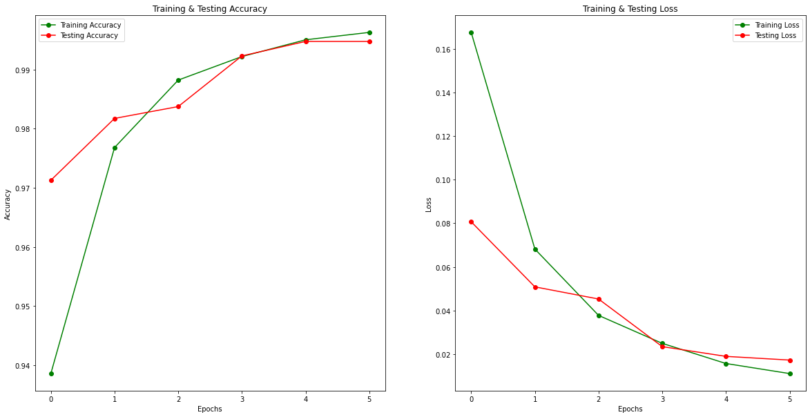
epochs = [i for i in range(6)]
fig , ax = plt.subplots(1,2)
train_acc = history.history['accuracy']
train_loss = history.history['loss']
val_acc = history.history['val_accuracy']
val_loss = history.history['val_loss']
fig.set_size_inches(20,10)

ax[0].plot(epochs , train_acc , 'go-' , label = 'Training Accuracy')
ax[0].plot(epochs , val_acc , 'ro-' , label = 'Testing Accuracy')
ax[0].set_title('Training & Testing Accuracy')
ax[0].legend()
ax[0].set_xlabel("Epochs")
ax[0].set_ylabel("Accuracy")

ax[1].plot(epochs , train_loss , 'go-' , label = 'Training Loss')
ax[1].plot(epochs , val_loss , 'ro-' , label = 'Testing Loss')
ax[1].set_title('Training & Testing Loss')
ax[1].legend()
ax[1].set_xlabel("Epochs")
ax[1].set_ylabel("Loss")
plt.show()

6. モデルの評価

我々のモデルは、テストデータセットにおいて99.48%の精度で非常に良好なパフォーマンスを示しています。

result = model.evaluate(X_test, y_test)
# extract those
loss = result[0]
accuracy = result[1]


print(f"[+] Accuracy: {accuracy*100:.2f}%")

281/281 [==============================] - 19s 69ms/step - loss: 0.0172 - accuracy: 0.9948
[+] Accuracy: 99.48%

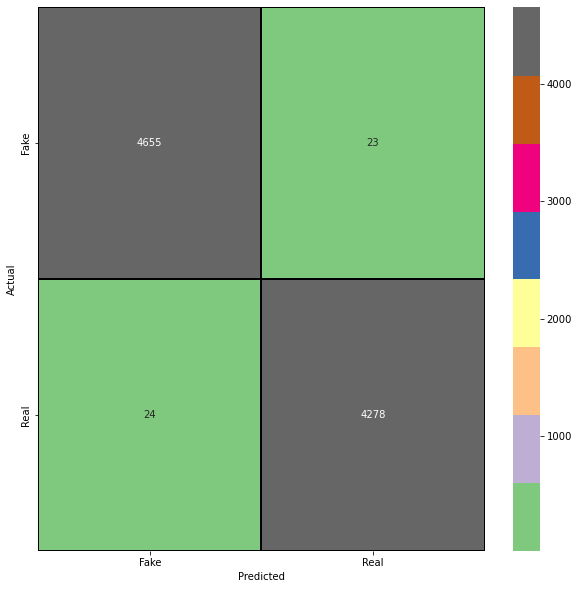
また、テストデータセットにおける我々のモデルの精度と再現率を分析するために、混同行列を作成します。これにより、モデル評価の偽陽性と偽陰性について、より深い洞察を得ることができます。

pred = model.predict_classes(X_test)
cm = confusion_matrix(y_test,pred)
cm = pd.DataFrame(cm , index = ['Fake','Real'] , columns = ['Fake','Real'])

plt.figure(figsize = (10,10))
sns.heatmap(cm,cmap= "Accent", linecolor = 'black' , linewidth = 1 , annot = True, fmt='' , xticklabels = ['Fake','Real'] , yticklabels = ['Fake','Real'])
plt.xlabel("Predicted")
plt.ylabel("Actual")

Text(69.0, 0.5, 'Actual')

7. 結論

このチュートリアルでは、NLPの技術とGridDBを使用して、非常に正確なフェイクニュース識別モデルを構築しました。データのインポート方法として、(1) GridDBと(2) Pandasの2つを検討しました。GridDBはオープンソースで拡張性が高いため、大規模なデータセットを扱う場合、ノートブックにデータを取り込むための優れた選択肢となります。GridDBを今すぐダウンロードしてください。