はじめに
今回は、TensorFlowJSとGridDBを使ってモデルを学習し、赤ワインの品質を予測します。このチュートリアルでは、以下のNodeJS用ライブラリを使用します。
- TensorflowJS - モデルのトレーニングに使用します。
- DanfoJS - DataFrameの操作に使用します。
記事の全コードはこちら をご覧ください。
データサイエンスやMLの実験を容易にするためにはNode Notebooksを使った作業が便利です。Visual Studio CodeはNode Notebooksをサポートする素晴らしいエディタなので、この記事ではそれを使用することにします。注: Danfo JS と Tensorflow JS は最低でもnodeのバージョン 12 が必要で、griddb はnodeのバージョン 10 で動きます。
const dfd = require("danfojs-node")
var fs     = require('fs');
const tf = dfd.tensorflow
const tfvis = require('@tensorflow/tfjs-vis')
使用するデータセットは、This Kaggle Datasetのものを使用する予定です。
まずは、データセットをCSVで読み込み、GridDBに挿入するところから始めます。
GridDBにデータをロードし、GridDBからデータをフェッチする
まず、GridDB サーバに接続します。同じマシン(localhost)上で動作させています。
var griddb = require('griddb_node');

const createCsvWriter = require('csv-writer').createObjectCsvWriter;
const csvWriter = createCsvWriter({
  path: 'out.csv',
  header: [
    {id: "fixed acidity", title:"fixed acidity"},
    {id: "volatile acidity", title:"volatile acidity"},
    {id: "citric acid", title:"citric acid"},
    {id: "residual sugar", title:"residual sugar"},
    {id: "chlorides", title:"chlorides"},
    {id: "free sulfur dioxide", title:"free sulfur dioxide"},
    {id: "total sulfur dioxide" , title:"total sulfur dioxide"},
    {id: "density", title:"density"},
    {id: "pH", title:"pH"},
    {id: "sulphates", title:"sulphates"},
    {id: "alcohol", title:"alcohol"},
    {id: "quality", title:"quality"}
  ]
});

const factory = griddb.StoreFactory.getInstance();
const store = factory.getStore({
    "host": '239.0.0.1',
    "port": 31999,
    "clusterName": "defaultCluster",
    "username": "admin",
    "password": "admin"
});
// For connecting to the GridDB Server we have to make containers and specify the schema.
const conInfo = new griddb.ContainerInfo({
    'name': "redwinequality",
    'columnInfoList': [
      ["name", griddb.Type.STRING],
      ["fixedacidity", griddb.Type.DOUBLE],
      ["volatileacidity", griddb.Type.DOUBLE],
      ["citricacid", griddb.Type.DOUBLE],
      ["residualsugar", griddb.Type.DOUBLE],
      ["chlorides", griddb.Type.DOUBLE],
      ["freesulfurdioxide", griddb.Type.INTEGER],
      ["totalsulfurdioxide", griddb.Type.INTEGER],
      ["density", griddb.Type.DOUBLE],
      ["pH", griddb.Type.DOUBLE],
      ["sulphates", griddb.Type.DOUBLE],
      ["alcohol", griddb.Type.DOUBLE],
      ["quality", griddb.Type.INTEGER],
    ],
    'type': griddb.ContainerType.COLLECTION, 'rowKey': true
});


// ////////////////////////////////////////////


const csv = require('csv-parser');

const fs = require('fs');
var lst = []
var lst2 = []
var i =0;
fs.createReadStream('./dataset/winequality-red.csv')
  .pipe(csv())
  .on('data', (row) => {
    lst.push(row);
  })
  .on('end', () => {

    var container;
    var idx = 0;

    for(let i=0;i<lst.length;i++){
        lst[i]["fixed acidity"] = parseFloat(lst[i]["fixed acidity"])

        lst[i]['volatile acidity'] = parseFloat(lst[i]["volatile acidity"])
        lst[i]['citric acid'] = parseFloat(lst[i]["citric acid"])
        lst[i]['residual sugar'] = parseFloat(lst[i]["residual sugar"])
        lst[i]['chlorides'] = parseFloat(lst[i]["chlorides"])
        lst[i]['free sulfur dioxide'] = parseInt(lst[i]["free sulfur dioxide"])
        lst[i]['total sulfur dioxide'] = parseInt(lst[i]["total sulfur dioxide"])
        lst[i]['density'] = parseFloat(lst[i]["density"])
        lst[i]['pH'] = parseFloat(lst[i]["pH"])
        lst[i]['sulphates'] = parseFloat(lst[i]["sulphates"])
        lst[i]['alcohol'] = parseFloat(lst[i]["alcohol"])
        lst[i]['quality'] = parseFloat(lst[i]["quality"])


        console.log(parseFloat(lst[i]["fixed acidity"]))
    store.putContainer(conInfo, false)
        .then(cont => {
            container = cont;
            return container.createIndex({ 'columnName': 'name', 'indexType': griddb.IndexType.DEFAULT });
        })
        .then(() => {
            idx++;
            container.setAutoCommit(false);
            return container.put([String(idx), lst[i]['fixed acidity'],lst[i]["volatile acidity"],lst[i]["citric acid"],lst[i]["residual sugar"],lst[i]["chlorides"],lst[i]["free sulfur dioxide"],lst[i]["total sulfur dioxide"],lst[i]["density"],lst[i]["pH"],lst[i]["sulphates"],lst[i]["alcohol"],lst[i]["quality"]]);
        })
        .then(() => {
            return container.commit();
        })

        .catch(err => {
            if (err.constructor.name == "GSException") {
                for (var i = 0; i < err.getErrorStackSize(); i++) {
                    console.log("[", i, "]");
                    console.log(err.getErrorCode(i));
                    console.log(err.getMessage(i));
                }
            } else {
                console.log(err);
            }
        });
    }
    store.getContainer("redwinequality")
    .then(ts => {
        container = ts;
      query = container.query("select *")
      return query.fetch();
  })
  .then(rs => {
      while (rs.hasNext()) {
          let rsNext = rs.next();
          lst2.push(

                {
                    'fixed acidity': rsNext[1],
                    "volatile acidity": rsNext[2],
                    "citric acid": rsNext[3],
                    "residual sugar": rsNext[4],
                    "chlorides": rsNext[5],
                    "free sulfur dioxide": rsNext[6],
                    "total sulfur dioxide": rsNext[7],
                    "density": rsNext[8],
                    "pH": rsNext[9],
                    "sulphates": rsNext[10],
                    "alcohol": rsNext[11],
                    "quality": rsNext[12]

                }


          );

      }


        csvWriter
        .writeRecords(lst2)
        .then(()=> console.log('The CSV file was written successfully'));


      return
  }).catch(err => {
      if (err.constructor.name == "GSException") {
          for (var i = 0; i < err.getErrorStackSize(); i++) {
              console.log("[", i, "]");
              console.log(err.getErrorCode(i));
              console.log(err.getMessage(i));
          }
      } else {
          console.log(err);
      }
  });

  });
そして、同じコードでGridDBからデータを取得し、csvファイルに書き込んでいます。このようにした理由は、プロジェクトファイルはnodeのバージョン12で動作し、GridDBのコードはnodeのバージョン10で動作するからです。
let df = await dfd.readCSV("./out.csv")
次に、node notebookでcsvファイルを読み込み、その上で探索的データ解析を行います。その後、前処理とモデリングに移行することができます。
GridDBから取得したデータをdfという変数に格納し、データフレームを作成しました。
探索的データ解析
EDAの段階では、データがどのようなものかを把握するために、データをチェックします。一番簡単なのは、何行あって、何列あって、それぞれの列のデータ型は何なのかを確認することです。
データフレームの形状を確認します。1599行と12列のデータであることがわかります。
console.log(df.shape)

//  Output
// [ 1599, 12 ]
では、列を確認します。それぞれの行に異なる数量が与えられています。そして、目標にする品質変数です。
出力
['fixed acidity','volatile acidity','citric acid','residual sugar','chlorides','free sulfur dioxide', 'total sulfur dioxide','density','pH','sulphates','alcohol','quality']
danfoJSのprint関数は最大10行の印刷が可能なので、列型の印刷は2回に分けて行わなければなりません。
df.loc({columns:['fixed acidity',
'volatile acidity',
'citric acid',
'residual sugar',
'chlorides',
'free sulfur dioxide','total sulfur dioxide',
'density']}).ctypes.print()

//  Output
// ╔══════════════════════╤═════════╗
// ║ fixed acidity        │ float32 ║
// ╟──────────────────────┼─────────╢
// ║ volatile acidity     │ float32 ║
// ╟──────────────────────┼─────────╢
// ║ citric acid          │ float32 ║
// ╟──────────────────────┼─────────╢
// ║ residual sugar       │ float32 ║
// ╟──────────────────────┼─────────╢
// ║ chlorides            │ float32 ║
// ╟──────────────────────┼─────────╢
// ║ free sulfur dioxide  │ int32   ║
// ╟──────────────────────┼─────────╢
// ║ total sulfur dioxide │ int32   ║
// ╟──────────────────────┼─────────╢
// ║ density              │ float32 ║
// ╚══════════════════════╧═════════╝
df.loc({columns:['pH',
'sulphates',
'alcohol',
'quality']}).ctypes.print()

//  Output

// ╔═══════════╤═════════╗
// ║ pH        │ float32 ║
// ╟───────────┼─────────╢
// ║ sulphates │ float32 ║
// ╟───────────┼─────────╢
// ║ alcohol   │ float32 ║
// ╟───────────┼─────────╢
// ║ quality   │ int32   ║
// ╚═══════════╧═════════╝
ここで、すべての列の統計の要約を見て、その最小値、最大値、平均値、標準偏差などを確認します。
df.loc({columns:['fixed acidity',
'volatile acidity',
'citric acid',
'residual sugar',
'chlorides',
'free sulfur dioxide','total sulfur dioxide',
'density']}).describe().round(2).print()

// Output
// ╔════════════╤═══════════════════╤═══════════════════╤═══════════════════╤═══════════════════╤═══════════════════╤═══════════════════╤═══════════════════╤═══════════════════╗
// ║            │ fixed acidity     │ volatile acidity  │ citric acid       │ residual sugar    │ chlorides         │ free sulfur dio…  │ total sulfur di…  │ density           ║
// ╟────────────┼───────────────────┼───────────────────┼───────────────────┼───────────────────┼───────────────────┼───────────────────┼───────────────────┼───────────────────╢
// ║ count      │ 1599              │ 1599              │ 1599              │ 1599              │ 1599              │ 1599              │ 1599              │ 1599              ║
// ╟────────────┼───────────────────┼───────────────────┼───────────────────┼───────────────────┼───────────────────┼───────────────────┼───────────────────┼───────────────────╢
// ║ mean       │ 8.32              │ 0.53              │ 0.27              │ 2.54              │ 0.09              │ 15.87             │ 46.47             │ 1                 ║
// ╟────────────┼───────────────────┼───────────────────┼───────────────────┼───────────────────┼───────────────────┼───────────────────┼───────────────────┼───────────────────╢
// ║ std        │ 1.74              │ 0.18              │ 0.19              │ 1.41              │ 0.05              │ 10.46             │ 32.9              │ 0                 ║
// ╟────────────┼───────────────────┼───────────────────┼───────────────────┼───────────────────┼───────────────────┼───────────────────┼───────────────────┼───────────────────╢
// ║ min        │ 4.6               │ 0.12              │ 0                 │ 0.9               │ 0.01              │ 1                 │ 6                 │ 0.99              ║
// ╟────────────┼───────────────────┼───────────────────┼───────────────────┼───────────────────┼───────────────────┼───────────────────┼───────────────────┼───────────────────╢
// ║ median     │ 7.9               │ 0.52              │ 0.26              │ 2.2               │ 0.08              │ 14                │ 38                │ 1                 ║
// ╟────────────┼───────────────────┼───────────────────┼───────────────────┼───────────────────┼───────────────────┼───────────────────┼───────────────────┼───────────────────╢
// ║ max        │ 15.9              │ 1.58              │ 1                 │ 15.5              │ 0.61              │ 72                │ 289               │ 1                 ║
// ╟────────────┼───────────────────┼───────────────────┼───────────────────┼───────────────────┼───────────────────┼───────────────────┼───────────────────┼───────────────────╢
// ║ variance   │ 3.03              │ 0.03              │ 0.04              │ 1.99              │ 0                 │ 109.41            │ 1082.1            │ 0                 ║
// ╚════════════╧═══════════════════╧═══════════════════╧═══════════════════╧═══════════════════╧═══════════════════╧═══════════════════╧═══════════════════╧═══════════════════╝
df.loc({columns:['pH','sulphates','alcohol','quality']}).describe().round(2).print()

// Output
// ╔════════════╤═══════════════════╤═══════════════════╤═══════════════════╤═══════════════════╗
// ║            │ pH                │ sulphates         │ alcohol           │ quality           ║
// ╟────────────┼───────────────────┼───────────────────┼───────────────────┼───────────────────╢
// ║ count      │ 1599              │ 1599              │ 1599              │ 1599              ║
// ╟────────────┼───────────────────┼───────────────────┼───────────────────┼───────────────────╢
// ║ mean       │ 3.31              │ 0.66              │ 10.42             │ 5.64              ║
// ╟────────────┼───────────────────┼───────────────────┼───────────────────┼───────────────────╢
// ║ std        │ 0.15              │ 0.17              │ 1.07              │ 0.81              ║
// ╟────────────┼───────────────────┼───────────────────┼───────────────────┼───────────────────╢
// ║ min        │ 2.74              │ 0.33              │ 8.4               │ 3                 ║
// ╟────────────┼───────────────────┼───────────────────┼───────────────────┼───────────────────╢
// ║ median     │ 3.31              │ 0.62              │ 10.2              │ 6                 ║
// ╟────────────┼───────────────────┼───────────────────┼───────────────────┼───────────────────╢
// ║ max        │ 4.01              │ 2                 │ 14.9              │ 8                 ║
// ╟────────────┼───────────────────┼───────────────────┼───────────────────┼───────────────────╢
// ║ variance   │ 0.02              │ 0.03              │ 1.14              │ 0.65              ║
// ╚════════════╧═══════════════════╧═══════════════════╧═══════════════════╧═══════════════════╝
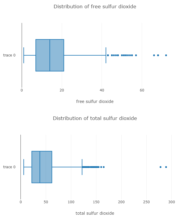
さて、分布を可視化するために、箱ひげ図とヒストグラムを使用します。
## Distribution of Column Values
const { Plotly } = require('node-kernel');
let cols = df.columns
for(let i = 0; i < cols.length; i++)
{
    let data = [{
        x: df[cols[i]].values,
        type: 'box'}];
    let layout = {
        height: 400,
        width: 700,
        title: 'Distribution of '+cols[i],
        xaxis: {title: cols[i]}};
    // There is no HTML element named `myDiv`, hence the plot is displayed below.
    Plotly.newPlot('myDiv', data, layout);
}
そして、ここに2つの列の箱ひげ図があります。
品質と他のカラムの散布図をプロットします。
## Scatter Plot between Wine Quality and Column
let cols = [...cols]
cols.pop('quality')
for(let i = 0; i < cols.length; i++)
{
    let data = [{
        x: df[cols[i]].values,
        y: df['quality'].values,
        type: 'scatter',
        mode: 'markers'}];
    let layout = {
        height: 400,
        width: 700,
        title: 'Red Wine Quality vs '+cols[i],
        xaxis: {title: cols[i]},
        yaxis: {title: 'Quality'}};
    // There is no HTML element named `myDiv`, hence the plot is displayed below.
    Plotly.newPlot('myDiv', data, layout);
}
2つの列の例に対するプロットは以下の通りです。
プロットを見ると、これらの列はワインの品質を予測するために使用することができ、間違いなくモデルを作ることができると言えるでしょう。
データの前処理
データはほとんど整理されているので、NULL値を削除するだけです。
df_drop = df.dropNa({ axis: 0 }).loc({columns:['quality','density']})
モデル
入力層と出力層を1つずつ持つ単純なニューラルネットワークを作成します。
function createModel() {
// Create a sequential model
const model = tf.sequential();
// Add a single input layer
model.add(tf.layers.dense({inputShape: [1], units: 10, useBias: true}));
// Add an output layer
model.add(tf.layers.dense({units: 1, useBias: true}));
return model;
}
// Create the model
const model = createModel();
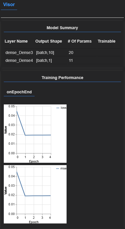
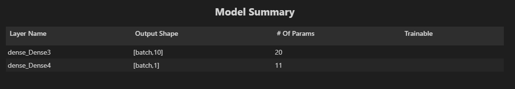
tfvis.show.modelSummary({name: 'Model Summary'}, model);
Model Summaryには、層と各層のニューロン数が表示されます。
モデルを作成したので、次にデータをテンソル形式に変換して、Tensorflowがモデルを学習できるようにする必要があります。
function convertToTensor(data) {
    // Wrapping these calculations in a tidy will dispose any
    // intermediate tensors.

    return tf.tidy(() => {
      // Step 1. Shuffle the data
      tf.util.shuffle(data);

      // Step 2. Convert data to Tensor
      const inputs = data.map(d => d[0]);
      const labels = data.map(d => d[1]);
      // console.log(inputs);
      // console.log(data);

      const inputTensor = tf.tensor2d(inputs, [inputs.length, 1]);
      const labelTensor = tf.tensor2d(labels, [labels.length, 1]);

      //Step 3. Normalize the data to the range 0 - 1 using min-max scaling
      const inputMax = inputTensor.max();
      const inputMin = inputTensor.min();
      const labelMax = labelTensor.max();
      const labelMin = labelTensor.min();

      const normalizedInputs = inputTensor.sub(inputMin).div(inputMax.sub(inputMin));
      const normalizedLabels = labelTensor.sub(labelMin).div(labelMax.sub(labelMin));

      return {
        inputs: normalizedInputs,
        labels: normalizedLabels,
        // Return the min/max bounds so we can use them later.
        inputMax,
        inputMin,
        labelMax,
        labelMin,
      }
    });


}
そして、モデルがどのように学習するかを指定する関数を作成します。ここでは、損失を予測値と実際の品質値の間の平均二乗誤差とします。
async function trainModel(model, inputs, labels) {
  // Prepare the model for training.
  model.compile({
    optimizer: "adam",
    loss: tf.losses.meanSquaredError,
    metrics: ['mse'],
  });

  const batchSize = 2;
  const epochs = 5;

  await model.fit(inputs, labels, {
    batchSize,
    epochs,
    shuffle: true,
    callbacks: tfvis.show.fitCallbacks(
      { name: 'Training Performance' },
      ['loss', 'mse'],
      { height: 200, callbacks: ['onEpochEnd'] }
    )
  });
  return model;
}
最後に、モデルを学習させます。デモのため、エポック数は5のみに設定しました。これはモデルやデータによって設定する必要があります。また、データセットの最初の100行はテスト用に残しておきます。
const tensorData = convertToTensor(df_drop.values)
const {inputs, labels} = tensorData;
// Train the model
let model = await trainModel(model, inputs.slice([100],[-1]), labels.slice([100],[-1]));
console.log('Done Training');

// Output
// Epoch 1 / 5
// Epoch 2 / 5
// Epoch 3 / 5
// Epoch 4 / 5
// Epoch 5 / 5
// Done Training


// 11819ms 7392us/step - loss=0.0450 mse=0.0450

// 10833ms 6775us/step - loss=0.0190 mse=0.0190

// 10878ms 6803us/step - loss=0.0192 mse=0.0192

// 10642ms 6655us/step - loss=0.0192 mse=0.0192

// 11025ms 6895us/step - loss=0.0193 mse=0.0193
モデルの学習が完了したので、モデルを評価することができます。評価にはevaluate関数を使用し、テストセット(学習時に残った最初の100行のデータセット)でモデルをテストすることができます。
model.evaluate(inputs.slice([0],[100]), labels.slice([0],[100]))[0].print() // Loss
model.evaluate(inputs.slice([0],[100]), labels.slice([0],[100]))[1].print() // Metric

// Output
// Tensor
    // 0.018184516578912735
今回は、TensorflowJSとGridDBを組み合わせてモデルを学習し、予測を行う方法を学びました。