はじめに
こんにちは、事業会社で働いているデータサイエンティストです。
本記事では、ディリクレ過程回帰モデルという、柔軟に独立変数(共変量、特徴量)と従属変数(結果変数)の関係性をモデリングする手法を紹介します。詳細はHannah, Blei and Powell(2011)を参照してください。
さて、ディリクレ過程回帰はノンパラメトリックベイズの一種なんですが、柔軟に独立変数と従属変数をモデリングする手法でいうとガウス過程で良いのでは?という疑問もあるかもしれません。
勉強不足の状態での個人的な意見になりますが、ガウス過程には二つの大きな課題があります:
- 独立変数と従属変数の関係を記憶する巨大な共分散行列の逆行列を求める必要があり、そもそもあまりスケールしません
- 曲線の当てはめに置き換えられるタスク以外で活用しにくい
一つ目の問題はEC2で強力なインスタンスを立ててそこで計算すればある程度解決できるが、本質的な計算量問題は避けられません。なので、個人的には計算量が限られる「時間と従属変数の関係」(10年分の日次データでも4000件に行かない)をモデリングする時しか使いません。
では、この重いガウス過程に代わる手法、ディリクレ過程回帰モデルの説明に入りますー
モデルの考え方の説明
ディリクレ過程回帰モデルの考えはとてもシンプルです。
要するに、似たような独立変数の値を取る観測値同士に焦点を絞ると、独立変数と従属変数の関係は線形モデルで記述できるという発想です。円形でも、ある点の近くをめっちゃくちゃ拡大すれば、ほぼ直線に見えるということです。概念的には微分に近いです。
この観測値の近傍の点から情報を取るのは重要な考えで、実はランダムフォレストも裏で同じことをしていることが知られています(Lin and Joen 2006)。
「近傍」をどう定義すればいいかに関して、ディリクレ過程回帰は、これをディリクレ過程によるクラスタリングで表現します。独立変数の値が同じクラスターに分類された観測値グループごと単純な線形モデルを作るということです。
次は実際この考えを確率モデルで記述します。
モデル定式化
まずは確率モデルを書きたいので、詳細の説明は下の方で行います。
- 全体のディリクレ過程
$$d\_alpha\sim Gamma(0.1, 0.1)$$
$$z\sim Stick\space Breaking(d\_alpha)$$
- 全クラスター共通のパラメーター
$$sigma_{y} \sim Gamma(0.1, 0.1)$$
- 全てのクラスターkについて
$$sigma_{x_{k}}\sim Gamma(0.1, 0.1)$$
$$sigma_{intercept_{k}}\sim Gamma(0.1, 0.1)$$
$$sigma_{beta_{k}}\sim Gamma(0.1, 0.1)$$
$$X_{latent_{k}}\sim Normal(0, 1)$$
$$intercept_{k}\sim Normal(0, 1/sigma_{intercept_{k}})$$
$$beta_{k}\sim Normal(0, 1/sigma_{beta_{k}})$$
- 観測値nについて
$$\eta_{n} \sim Categorical(z)$$
$$X_{n} \sim Normal(X_{latent_{\eta_{n}}}, 1/sigma_{x_{\eta_{n}}})$$
$$Y_{n} \sim Normal(intercept_{\eta_{n}} + X_{n} * beta_{\eta_{n}}, 1/sigma_{y})$$
$X_{latent_{k}}$が要するにk番目のクラスターのXの平均だと理解しても問題ないです。
切片(intercept)と傾き(beta)は所属クラスターによって異なる値を取ります。
ここで強調しておきたいのは、Stanは離散確率変数に従うパラメーターに対応していないので、$\eta_{n}$は計算時に積分除去され、事後分布を計算する時に再現されます。
$\eta$を再現する方法はこちらの記事を参照してください:
モデル実装
下記のStanのコードでモデルを実装できます。
予測の部分は、$\eta$の事後分布で各クラスターのパラメータ(interceptとbeta)の加重平均を取ることで行います。
data {
  int P;
  int N;
  int N_full;

  array[N] real x;
  array[N] real y;

  array[N_full] real x_full;
}
parameters {
  real<lower=0> d_alpha;                                       // ディリクレ過程の全体のパラメータ
  vector<lower=0, upper=1>[P - 1] breaks;  // ディリクレ過程のstick-breaking representationのためのパラメータ

  real<lower=0> sigma_y;
  vector<lower=0>[P] sigma_x;
  vector<lower=0>[P] sigma_intercept;
  vector<lower=0>[P] sigma_beta;
  vector[P] x_latent;
  vector[P] intercept;
  vector[P] beta;
}
transformed parameters {
  simplex[P] z; //
  {
    // stick-breaking representationの変換開始
    // https://discourse.mc-stan.org/t/better-way-of-modelling-stick-breaking-process/2530/2 を参考
    z[1] = breaks[1];
    real sum = z[1];
    for (p in 2:(P - 1)) {
      z[p] = (1 - sum) * breaks[p];
      sum += z[p];
    }
    z[P] = 1 - sum;
  }
}
model {
  d_alpha ~ gamma(0.1, 0.1);

  breaks ~ beta(1, d_alpha);

  sigma_y ~ gamma(0.1, 0.1);
  sigma_x ~ gamma(0.1, 0.1);
  sigma_intercept ~ gamma(0.1, 0.1);
  sigma_beta ~ gamma(0.1, 0.1);
  x_latent ~ normal(0, 1);
  intercept ~ normal(0, 1/sigma_intercept);
  beta ~ normal(0, 1/sigma_beta);

  for (i in 1:N){
    // etaの積分除去処理開始
    vector[P] case_vector;
    for (p in 1:P){
      case_vector[p] = log(z[p]) +
                       normal_lupdf(x[i] | x_latent[p], 1/sigma_x[p]) +
                       normal_lupdf(y[i] | intercept[p] + x[i] * beta[p], sigma_y);
    }
    target += log_sum_exp(case_vector);
    // etaの積分除去処理終了
  }
}
generated quantities {
  array[N_full] vector[P] eta;
  array[N_full] real y_predicted;

  for (i in 1:N_full){
    // ベイズ定理でetaの事後分布を計算
    vector[P] case_vector;
    for (p in 1:P){
      case_vector[p] = z[p] * exp(
        normal_lpdf(x_full[i] | x_latent[p], 1/sigma_x[p])
      );
    }
    eta[i] = case_vector./sum(case_vector);
    y_predicted[i] = normal_rng(intercept '* eta[i] + x_full[i] * (beta '* eta[i]), sigma_y);
  }
}
モデル推定
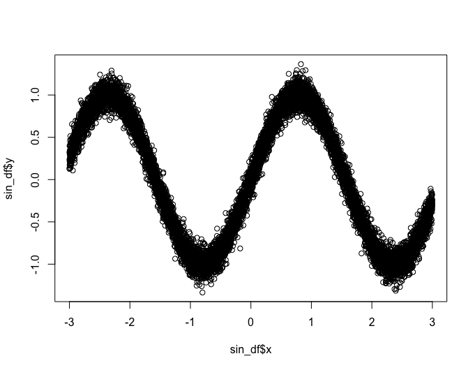
今回ディリクレ過程回帰に学習させるのは、ノイズ入りのsin関数
set.seed(12345)

sin_df <- tibble::tibble(
  x = seq(from = -3, to = 3, length.out = 10000)
) |>
  dplyr::mutate(
    e = rnorm(dplyr::n(), sd = 0.1),
    y = sin(2 * x) + e,
    x_std = (x - mean(x))/sd(x),
    train = dplyr::case_when(
      dplyr::between(x, -2.75, 2.75) ~ "train",
      TRUE ~ "test"
    )
  )
plot(sin_df$x, sin_df$y)
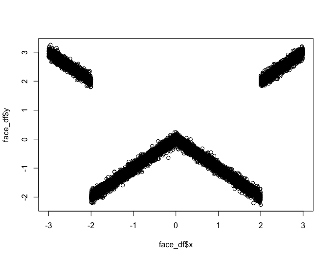
と「日付データに『2024年3月です』(全角)が入っているレコードを見たデータサイエンティストの顔」関数です。
set.seed(12345)

face_df <- tibble::tibble(
  x = seq(from = -3, to = 3, length.out = 10000)
) |>
  dplyr::mutate(
    e = rnorm(dplyr::n(), sd = 0.1),
    y = dplyr::case_when(
      x < -2 ~ -1 * x + e,
      dplyr::between(x, -2, 0) ~ 1 * x + e,
      dplyr::between(x, 0, 2) ~ -1 * x + e,
      TRUE ~ 1 * x + e
    ),
    x_std = (x - mean(x))/sd(x),
    train = dplyr::case_when(
      dplyr::between(x, -2.75, 2.75) ~ "train",
      TRUE ~ "test"
    )
  )
plot(face_df$x, face_df$y)
Xが-2.75と2.75の間にあるデータは学習データになり、その他のデータは検証データになります。
ではそれぞれ学習を行いましょう!
まずはsin関数から:
sin_data_list <- list(
  P = 10,
  N = sum(sin_df$train == "train"),
  N_full = nrow(sin_df),

  x = sin_df$x_std[which(sin_df$train == "train")],
  y = sin_df$y[which(sin_df$train == "train")],

  x_full = sin_df$x_std
)

m_dr_sin_init <- cmdstanr::cmdstan_model("dirichlet_regression.stan")
> m_dr_sin_estimate <- m_dr_sin_init$variational(
     data = sin_data_list,
     seed = 12345
 )
------------------------------------------------------------
EXPERIMENTAL ALGORITHM:
  This procedure has not been thoroughly tested and may be unstable
  or buggy. The interface is subject to change.
------------------------------------------------------------
Gradient evaluation took 0.019825 seconds
1000 transitions using 10 leapfrog steps per transition would take 198.25 seconds.
Adjust your expectations accordingly!
Begin eta adaptation.
Iteration:   1 / 250 [  0%]  (Adaptation)
Iteration:  50 / 250 [ 20%]  (Adaptation)
Iteration: 100 / 250 [ 40%]  (Adaptation)
Iteration: 150 / 250 [ 60%]  (Adaptation)
Iteration: 200 / 250 [ 80%]  (Adaptation)
Success! Found best value [eta = 1] earlier than expected.
Begin stochastic gradient ascent.
  iter             ELBO   delta_ELBO_mean   delta_ELBO_med   notes
   100       -12697.946             1.000            1.000
   200        -8512.918             0.746            1.000
   300        -7515.912             0.541            0.492
   400        -7292.848             0.414            0.492
   500        -6627.024             0.351            0.133
   600        -6386.739             0.299            0.133
   700        -6111.456             0.263            0.100
   800        -6255.478             0.233            0.100
   900        -6149.604             0.209            0.045
  1000        -6018.570             0.190            0.045
  1100        -5888.490             0.092            0.038
  1200        -5995.123             0.045            0.031
  1300        -5956.945             0.032            0.023
  1400        -5803.710             0.032            0.023
  1500        -5986.975             0.025            0.023
  1600        -5891.760             0.023            0.022
  1700        -5966.567             0.019            0.022
  1800        -5881.724             0.019            0.018
  1900        -5824.072             0.018            0.018
  2000        -5757.343             0.017            0.016
  2100        -5739.553             0.015            0.014
  2200        -5724.534             0.013            0.013
  2300        -5745.948             0.013            0.013
  2400        -5741.875             0.011            0.012
  2500        -7052.954             0.026            0.012
  2600        -5952.304             0.043            0.012
  2700        -5951.875             0.042            0.010   MEDIAN ELBO CONVERGED
Drawing a sample of size 1000 from the approximate posterior...
COMPLETED.
Finished in  65.8 seconds.
m_dr_sin_summary <- m_dr_sin_estimate$summary()
データ量の割に計算がすぐ終わりました。
次は「日付データに『2024年3月です』(全角)が入っているレコードを見たデータサイエンティストの顔」関数です:
face_data_list <- list(
  P = 10,
  N = sum(face_df$train == "train"),
  N_full = nrow(face_df),

  x = face_df$x_std[which(face_df$train == "train")],
  y = face_df$y[which(face_df$train == "train")],

  x_full = face_df$x_std
)

m_dr_face_init <- cmdstanr::cmdstan_model("dirichlet_regression.stan")
> m_dr_face_estimate <- m_dr_face_init$variational(
     data = face_data_list,
     seed = 12345
 )
------------------------------------------------------------
EXPERIMENTAL ALGORITHM:
  This procedure has not been thoroughly tested and may be unstable
  or buggy. The interface is subject to change.
------------------------------------------------------------
Gradient evaluation took 0.018166 seconds
1000 transitions using 10 leapfrog steps per transition would take 181.66 seconds.
Adjust your expectations accordingly!
Begin eta adaptation.
Iteration:   1 / 250 [  0%]  (Adaptation)
Iteration:  50 / 250 [ 20%]  (Adaptation)
Iteration: 100 / 250 [ 40%]  (Adaptation)
Iteration: 150 / 250 [ 60%]  (Adaptation)
Iteration: 200 / 250 [ 80%]  (Adaptation)
Success! Found best value [eta = 1] earlier than expected.
Begin stochastic gradient ascent.
  iter             ELBO   delta_ELBO_mean   delta_ELBO_med   notes
   100        -8368.759             1.000            1.000
   200        -6729.424             0.622            1.000
   300        -6456.826             0.429            0.244
   400        -6023.923             0.339            0.244
   500        -4901.183             0.317            0.229
   600        -4274.338             0.289            0.229
   700        -4308.354             0.249            0.147
   800        -4328.028             0.218            0.147
   900        -4127.583             0.199            0.072
  1000        -4311.312             0.184            0.072
  1100        -4420.783             0.086            0.049
  1200        -4261.040             0.066            0.043
  1300        -4232.376             0.062            0.043
  1400        -4031.423             0.060            0.043
  1500        -4084.956             0.038            0.037
  1600        -4249.070             0.027            0.037
  1700        -4124.754             0.030            0.037
  1800        -3983.280             0.033            0.037
  1900        -4143.387             0.032            0.037
  2000        -4067.111             0.029            0.036
  2100        -4348.103             0.033            0.037
  2200        -4022.054             0.038            0.039
  2300        -4094.631             0.039            0.039
  2400        -3938.451             0.038            0.039
  2500        -7012.500             0.080            0.039
  2600        -5634.080             0.101            0.040
  2700        -5163.969             0.107            0.065
  2800        -3947.173             0.134            0.081
  2900        -4001.789             0.132            0.081
  3000        -4029.430             0.131            0.081
  3100        -4204.663             0.128            0.081
  3200        -3974.679             0.126            0.058
  3300        -3933.880             0.125            0.058
  3400        -3941.040             0.121            0.058
  3500        -3903.545             0.079            0.042
  3600        -3932.236             0.055            0.014
  3700        -3900.196             0.047            0.010
  3800        -3951.463             0.017            0.010
  3900        -4522.136             0.028            0.010
  4000        -3958.931             0.042            0.013
  4100        -3990.943             0.038            0.010
  4200        -4059.274             0.034            0.010
  4300        -3931.462             0.037            0.013
  4400        -3974.583             0.037            0.013
  4500        -4115.562             0.040            0.017
  4600        -3928.744             0.044            0.033
  4700        -4061.370             0.046            0.033
  4800        -3861.752             0.050            0.034
  4900        -3974.026             0.040            0.033
  5000        -3922.214             0.028            0.033
  5100        -4187.505             0.033            0.033
  5200        -3966.241             0.037            0.034
  5300        -3893.247             0.036            0.034
  5400        -3937.458             0.036            0.034
  5500        -4010.419             0.034            0.033
  5600        -3988.954             0.030            0.028
  5700        -4042.979             0.028            0.019
  5800        -4073.357             0.023            0.018
  5900        -3992.882             0.023            0.018
  6000        -3894.985             0.024            0.019
  6100        -3953.532             0.019            0.018
  6200        -4023.987             0.015            0.018
  6300        -3929.214             0.016            0.018
  6400        -3896.314             0.015            0.018
  6500        -3924.250             0.014            0.015
  6600       -11042.748             0.078            0.018
  6700        -3933.619             0.258            0.020
  6800        -3992.271             0.258            0.020
  6900        -3991.735             0.256            0.018
  7000        -3914.531             0.256            0.018
  7100        -3907.563             0.255            0.018
  7200        -3881.897             0.253            0.015
  7300        -3867.825             0.251            0.008   MEDIAN ELBO CONVERGED
Drawing a sample of size 1000 from the approximate posterior...
COMPLETED.
Finished in  132.0 seconds.
m_dr_face_summary <- m_dr_face_estimate$summary()
「日付データに『2024年3月です』(全角)が入っているレコードを見たデータサイエンティストの顔」関数は形が複雑怪奇なため、学習時間が少し長くなったが、こちらも2分ほどで終わりました。
可視化
性能を確認するため、まずは可視化しましょう!
g_sin <- m_dr_sin_summary |>
  dplyr::filter(stringr::str_detect(variable, "y_predicted")) |>
  dplyr::bind_cols(
    x = sin_df$x,
    y = sin_df$y,
    train = sin_df$train
  ) |>
  ggplot2::ggplot() +
  ggplot2::geom_point(ggplot2::aes(x = x, y = y, color = train)) +
  ggplot2::geom_line(ggplot2::aes(x = x, y = mean)) +
  ggplot2::geom_ribbon(ggplot2::aes(x = x, ymin = q5, ymax = q95),
                       fill = ggplot2::alpha("blue", 0.3)) +
  ggplot2::ggtitle("sin関数") +
  ggplot2::theme_gray(base_family = "HiraKakuPro-W3")

g_face <- m_dr_face_summary |>
  dplyr::filter(stringr::str_detect(variable, "y_predicted")) |>
  dplyr::bind_cols(
    x = face_df$x,
    y = face_df$y,
    train = face_df$train
  ) |>
  ggplot2::ggplot() +
  ggplot2::geom_point(ggplot2::aes(x = x, y = y, color = train)) +
  ggplot2::geom_line(ggplot2::aes(x = x, y = mean)) +
  ggplot2::geom_ribbon(ggplot2::aes(x = x, ymin = q5, ymax = q95),
                       fill = ggplot2::alpha("blue", 0.3)) +
  ggplot2::ggtitle("日付データに『2024年3月です』(全角)\nが入っているレコードを見たデータサイエンティストの顔") +
  ggplot2::theme_gray(base_family = "HiraKakuPro-W3")
gridExtra::grid.arrange(g_sin, g_face, nrow = 1)
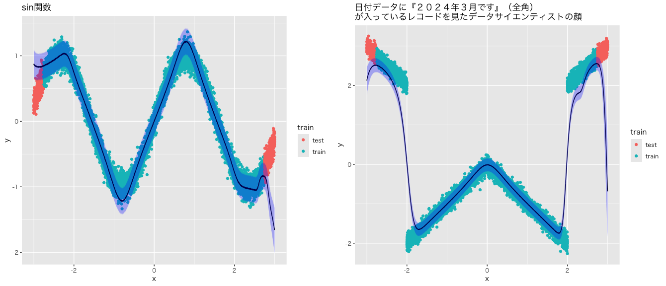
感覚的にはよくできていますが、検証データの区間で予測区間と実際のYの値に大きな乖離がありますが、そもそもデータ構造に関する事前知識を与えない状態での外挿はうまく行かないことが多いので、仕方ないです。
次に、特に左側のsin関数に着目していただきたいですが、sin関数の滑らかな曲線をディリクレ過程回帰モデルが直線で表現していることがわかります。クラスター(値が近しいXのグループ)ごとに線形モデルを当てはめるモデルがもたらした結果になります。
最後に、「日付データに『2024年3月です』(全角)が入っているレコードを見たデータサイエンティストの顔」関数はXが-2と2になるところの離散的な変化を見た目上きれいに表しているとは言えないですが、Yの値の大きなジャンプは学習できていると思います。
結論
いかがでしたか?
このように、ディリクレ過程はデータの複雑な構造を柔軟に学習できます。
次の記事では、ディリクレ過程モデルを因果推論の異質処置効果の推定に応用する手法を提案します。
参考文献
Hannah, Lauren A., David M. Blei, and Warren B. Powell. "Dirichlet process mixtures of generalized linear models." Journal of Machine Learning Research 12.6 (2011).
Lin, Yi, and Yongho Jeon. "Random forests and adaptive nearest neighbors." Journal of the American Statistical Association 101.474 (2006): 578-590.