はじめに
こんにちは、事業会社で働いているデータサイエンティストです。
本記事では、検証データに対して一部誤差率0.5%以下という高い精度を達成した多変量時系列モデル、ベイズファクターモデルを紹介します。
ファクターモデルとは
ファフターモデルは機械学習の世界で有名なembeddingモデル系と発想が極めて似ています。
まずembeddingモデルの代表のword2vecの復習から入りましょう。
word2vecの場合、対象の単語の埋め込み表現と周囲の文脈の単語の埋め込み表現の内積で対象の単語の出現を予測します。要するにこんな感じです
もちろん、活性化関数とか細かい内容もありますが、省略させてください。
ファフターモデルの場合、時系列の変数に埋め込み表現と時間の埋め込み表現がそれぞれ設定され、例えば鉄道駅の利用者数の時系列分析をする際、新宿駅の2024年4月1日の利用者数は
$$駅埋め込み表現_{新宿駅} '* 時間埋め込み表現_{2024年4月1日}$$
で表現されます。活性化関数などは省略します。
要するに、我々の手元にあるデータは、実はK個(埋め込み次元数)の見えない隠れ時系列の線形関係で表現できるということです。
図で表すと下記のようになります:
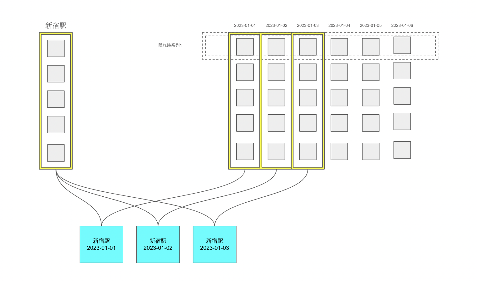
時系列分析問題をこのようにembedding系の手法に置き換えることで、大量の時系列の中に隠された相関とトレンドを効率よく学習することができ、高い予測性能が期待されます。
本記事が紹介する手法の理論的なところに興味ある方はBai and Wang(2015)をぜひ読んでみてください。
なお、本記事では、隠れ時系列、時間の埋め込み、ファクターを同義語として使います。
提案手法の紹介
時系列変数の埋め込み
時系列の埋め込みに関しては、仮説として、一部ノイズが強く、あまり質の良い情報を引き出せない変数もあります。なので、本手法は、馬蹄分布を事前分布として設定し、説明力の弱い変数の埋め込み表現が0付近になるようにします。
時間の埋め込み
時間の埋め込みに関しては、ベクトル自己回帰のモデル構造を設定します。
観測できない隠れ時系列に計量マクロ経済学でお馴染みのベクトル自己回帰を設定するだけです。
さらに、過去のXヶ月前の情報の重要度は埋め込み次元によって変わらないという情報を、馬蹄分布で表します。
例えば、ビジネスの場合、よく昨対比(さくたいひ)という表現を使いますが、これは要するに12ヶ月前のデータが今月のデータの状況をよく表すという事前情報です。
モデルの定式化
少し数学的な表現になりますが、本記事で提案するモデルはこのように定式化できます:
- 全体
$$sigma\sim Gamma(5, 5)$$
- 時系列変数
$$tau\space lambda\sim Cauchy(0, 1)$$
全ての時系列変数iについて
$$rho\space lambda_{i}\sim Cauchy(0, 1)$$
$$lambda_{i}\sim Normal(0, tau\space lambda * rho\space lambda_{i})$$
- 時間
$$tau\space lag\sim Cauchy(0, 1)$$
全てのラグ数iについて
$$rho\space lag_{i}\sim Cauchy(0, 1)$$
$$A_{i}\sim Normal(0, tau\space lag * rho\space lag_{i})$$
iを1から最大の時間まで
$$F_{i}\sim Normal(A_{1} * F_{i - 1} + A_{2} * F_{i - 2} + ... + A_{最大ラグ数} * F_{i - 最大ラグ数}, 1)$$
- 観測値
全ての観測値iについて
$$value_{i}\sim Normal(lambda_{時系列変数_{i}} '* F_{時間_{i}}, 1/sigma)$$
モデル実装
Stanでの実装はこんな感じです:
functions {
  real partial_sum_lpdf(
    array[] real value,
    int start, int end,

    array[] int series, array[] int time,

    real sigma,
    matrix F, matrix lambda
  ){
    vector[end - start + 1] log_likelihood;
    int count = 1;
    for (i in start:end){
      log_likelihood[count] = normal_lupdf(value[count] | F[time[i],] * lambda[series[i],]', 1/sigma);
      count += 1;
    }
    return sum(log_likelihood);
  }
}
data {
  int series_type;
  int time_type;
  int lag;
  int K;

  int N;
  array[N] int series;
  array[N] int time;
  array[N] real value;

  int N_full;
  array[N_full] int series_full;
  array[N_full] int time_full;
  vector[N_full] value_mean;
  vector[N_full] value_sd;
}
parameters {
  real<lower=0> sigma;

  matrix[time_type, K] F;

  real<lower=0> tau_lambda;
  vector<lower=0>[series_type] rho_lambda;
  matrix[series_type, K] lambda;

  real<lower=0> tau_lag;
  vector<lower=0>[lag] rho_lag;
  array[lag] matrix[K, K] A;
}
model {
  sigma ~ gamma(5, 5);

  tau_lambda ~ cauchy(0, 1);
  rho_lambda ~ cauchy(0, 1);

  tau_lag ~ cauchy(0, 1);
  rho_lag ~ cauchy(0, 1);

  for (i in 1:series_type){
    to_vector(lambda[i,]) ~ normal(0, tau_lambda * rho_lambda[i]);
  }

  for (i in 1:lag){
    to_vector(A[i]) ~ normal(0, tau_lag * rho_lag[i]);
  }

  to_vector(F[1:lag,]) ~ normal(0, 1);

  for (i in (lag + 1):time_type){
    row_vector[K] this_F = rep_vector(0.0, K)';
    for (j in 1:lag){
      this_F += F[i - j] * A[j];
    }
    F[i,] ~ normal(this_F, 1);
  }

  int grainsize = 1;

  target += reduce_sum(
    partial_sum_lupdf, value, grainsize,

    series, time,

    sigma,
    F, lambda
  );
}
generated quantities {
  vector[N_full] value_predicted;
  for (i in 1:N_full){
    value_predicted[i] = normal_rng((F[time_full[i],] * lambda[series_full[i],]' * value_sd[i]) + value_mean[i], 1/sigma);
  }
}
前処理
本記事では、アメリカのマクロ経済に関連する大量の時系列データを利用します。
> data(fred_md, package = "BVAR")
> fred_md |>
     tibble::rownames_to_column(var = "month") |>
     tibble::tibble()
# A tibble: 769 × 119
   month      RPI W875RX1 DPCERA3M086SBEA CMRMTSPLx RETAILx INDPRO IPFPNSS IPFINAL IPCONGD IPDCONGD IPNCONGD IPBUSEQ IPMAT IPDMAT IPNMAT IPMANSICS IPB51222S IPFUELS CUMFNS   HWI HWIURATIO
   <chr>    <dbl>   <dbl>           <dbl>     <dbl>   <dbl>  <dbl>   <dbl>   <dbl>   <dbl>    <dbl>    <dbl>   <dbl> <dbl>  <dbl>  <dbl>     <dbl>     <dbl>   <dbl>  <dbl> <int>     <dbl>
 1 1959-01… 2442.   2293.            17.3   292266.  18236.   22.0    23.4    22.3    31.6     18.7     38.2    8.15  20.1   12.1   30.7      20.9      19.9    34.7   80.2  1357     0.334
 2 1959-02… 2452.   2302.            17.5   294425.  18370.   22.4    23.7    22.5    31.8     18.8     38.5    8.26  20.8   12.7   31.2      21.3      19.9    34.2   81.4  1421     0.358
 3 1959-03… 2468.   2318.            17.6   293419.  18523.   22.8    23.9    22.6    31.8     19.2     38.3    8.35  21.3   13.2   31.7      21.6      20.0    35.1   82.5  1524     0.401
 4 1959-04… 2484.   2335.            17.6   299323.  18534.   23.3    24.2    22.9    32.3     19.3     39.0    8.56  21.9   13.6   32.6      22.1      20.1    34.9   84.0  1589     0.445
 5 1959-05… 2498.   2350.            17.8   301364.  18680.   23.6    24.4    23.1    32.5     19.7     39.0    8.84  22.5   14.1   32.9      22.4      20.4    34.2   84.9  1655     0.476
 6 1959-06… 2506.   2357.            17.8   301349.  18850.   23.6    24.6    23.3    32.3     19.8     38.7    9.05  22.3   14.0   32.8      22.4      20.5    34.2   84.8  1717     0.501
 7 1959-07… 2504.   2356.            17.8   305020.  18844.   23.1    24.6    23.5    32.7     20.2     39.0    9.07  21.0   12.6   33.0      22.0      20.8    33.5   83.0  1723     0.488
 8 1959-08… 2490.   2342.            17.9   289435.  18964.   22.3    24.4    23.4    32.8     19.6     39.5    8.99  19.4   11.0   32.9      21.1      20.9    34.0   79.5  1638     0.457
 9 1959-09… 2492.   2342.            18.1   293698.  18716.   22.3    24.3    23.4    32.7     19.1     39.7    8.92  19.4   11.0   32.9      21.1      21.3    33.8   79.0  1605     0.425
10 1959-10… 2495.   2345.            17.9   294168.  18853.   22.1    24.3    23.3    32.5     19.5     39.2    8.85  19.2   10.8   32.3      20.9      21.4    33.6   78.2  1553     0.397
# ℹ 759 more rows
# ℹ 97 more variables: CLF16OV <int>, CE16OV <int>, UNRATE <dbl>, UEMPMEAN <dbl>, UEMPLT5 <int>, UEMP5TO14 <int>, UEMP15OV <int>, UEMP15T26 <int>, UEMP27OV <int>, CLAIMSx <int>,
#   PAYEMS <int>, USGOOD <int>, CES1021000001 <dbl>, USCONS <int>, MANEMP <int>, DMANEMP <int>, NDMANEMP <int>, SRVPRD <int>, USTPU <int>, USWTRADE <dbl>, USTRADE <dbl>, USFIRE <int>,
#   USGOVT <int>, CES0600000007 <dbl>, AWOTMAN <dbl>, AWHMAN <dbl>, HOUST <int>, HOUSTNE <int>, HOUSTMW <int>, HOUSTS <int>, HOUSTW <int>, PERMIT <int>, PERMITNE <int>, PERMITMW <int>,
#   PERMITS <int>, PERMITW <int>, ACOGNO <int>, AMDMNOx <dbl>, ANDENOx <dbl>, AMDMUOx <dbl>, BUSINVx <dbl>, ISRATIOx <dbl>, M1SL <dbl>, M2SL <dbl>, M2REAL <dbl>, BOGMBASE <int>,
#   TOTRESNS <dbl>, NONBORRES <int>, BUSLOANS <dbl>, REALLN <dbl>, NONREVSL <dbl>, CONSPI <dbl>, FEDFUNDS <dbl>, CP3Mx <dbl>, TB3MS <dbl>, TB6MS <dbl>, GS1 <dbl>, GS5 <dbl>, GS10 <dbl>,
#   COMPAPFFx <dbl>, TB3SMFFM <dbl>, TB6SMFFM <dbl>, T1YFFM <dbl>, T5YFFM <dbl>, T10YFFM <dbl>, AAAFFM <dbl>, EXSZUSx <dbl>, EXJPUSx <dbl>, EXUSUKx <dbl>, EXCAUSx <dbl>, …
# ℹ Use `print(n = ...)` to see more rows
変数はかなり多いため、具体的な定義は省略します。詳細に興味ある方は下記のリンクを確認してください。Read Full Textの中のPDFの最後のところに説明があります。
これだとデータ分析と可視化の作業がめんどくさくなるので、データベース形式に変形して、値を標準化します:
freq_df <- fred_md |>
  tibble::rownames_to_column(var = "month") |>
  tibble::tibble() |>
  tidyr::pivot_longer(!month, names_to = "series", values_to = "value") |>
  tidyr::drop_na() |>
  dplyr::group_by(series) |>
  dplyr::mutate(
    value_std = (value - mean(value))/sd(value)
  ) |>
  dplyr::ungroup()
処理の結果はこんな感じです:
> freq_df
# A tibble: 90,010 × 4
   month      series             value value_std
   <chr>      <chr>              <dbl>     <dbl>
 1 1959-01-01 RPI               2442.      -1.39
 2 1959-01-01 W875RX1           2293.      -1.43
 3 1959-01-01 DPCERA3M086SBEA     17.3     -1.37
 4 1959-01-01 CMRMTSPLx       292266.      -1.41
 5 1959-01-01 RETAILx          18236.      -1.10
 6 1959-01-01 INDPRO              22.0     -1.68
 7 1959-01-01 IPFPNSS             23.4     -1.76
 8 1959-01-01 IPFINAL             22.3     -1.74
 9 1959-01-01 IPCONGD             31.6     -2.00
10 1959-01-01 IPDCONGD            18.7     -1.63
# ℹ 90,000 more rows
# ℹ Use `print(n = ...)` to see more rows
次に、マスター表を作成して、元データに結合します:
month_master <- freq_df |>
  dplyr::select(month) |>
  dplyr::distinct() |>
  dplyr::arrange(month) |>
  dplyr::mutate(
    month_id = dplyr::row_number()
  )

series_master <- freq_df |>
  dplyr::group_by(series) |>
  dplyr::summarise(
    # 標準化から元の状態に戻す処理もStanで実施するため、
    # 元に戻すために必要な時系列の平均値と標準偏差も持たせます
    value_mean = mean(value),
    value_sd = sd(value)
  ) |>
  dplyr::ungroup() |>
  dplyr::mutate(
    series_id = dplyr::row_number()
  )

freq_df_with_id <- freq_df |>
  dplyr::left_join(month_master, by = "month") |>
  dplyr::left_join(series_master, by = "series")
最後に、2023年1月を検証期間、残りの期間を学習期間にして、Stanに入れるためのリストを作成します:
freq_df_with_id_train <- freq_df_with_id |>
  dplyr::filter(as.Date(month) < as.Date("2023-01-01"))

fm_data_list <- list(
  series_type = nrow(series_master),
  time_type = nrow(month_master),
  lag = 24,
  K = 20,

  N = nrow(freq_df_with_id_train),
  series = freq_df_with_id_train$series_id,
  time = freq_df_with_id_train$month_id,
  value = freq_df_with_id_train$value_std,

  N_full = nrow(freq_df_with_id),
  series_full = freq_df_with_id$series_id,
  time_full = freq_df_with_id$month_id,
  value_mean = freq_df_with_id$value_mean,
  value_sd = freq_df_with_id$value_sd
)
モデル推定
では早速モデル推定を実施しましょう:
m_fm_init <- cmdstanr::cmdstan_model("factor_model.stan",
                                     cpp_options = list(
                                       stan_threads = TRUE
                                     )
                                     )
> m_fm_estimate <- m_fm_init$variational(
     seed = 123,
     threads = 10,
     iter = 10000,
     data = fm_data_list
 )
------------------------------------------------------------
EXPERIMENTAL ALGORITHM:
  This procedure has not been thoroughly tested and may be unstable
  or buggy. The interface is subject to change.
------------------------------------------------------------
Gradient evaluation took 0.082193 seconds
1000 transitions using 10 leapfrog steps per transition would take 821.93 seconds.
Adjust your expectations accordingly!
Begin eta adaptation.
Iteration:   1 / 250 [  0%]  (Adaptation)
Iteration:  50 / 250 [ 20%]  (Adaptation)
Iteration: 100 / 250 [ 40%]  (Adaptation)
Iteration: 150 / 250 [ 60%]  (Adaptation)
Iteration: 200 / 250 [ 80%]  (Adaptation)
Iteration: 250 / 250 [100%]  (Adaptation)
Success! Found best value [eta = 0.1].
Begin stochastic gradient ascent.
  iter             ELBO   delta_ELBO_mean   delta_ELBO_med   notes
   100     -4193500.981             1.000            1.000
   200      -866611.556             2.419            3.839
   300      -292951.149             2.266            1.958
   400      -199032.629             1.817            1.958
   500      -167398.522             1.492            1.000
   600      -144742.300             1.269            1.000
   700      -127139.343             1.108            0.472
   800      -113434.299             0.984            0.472
   900      -103125.225             0.886            0.189
  1000       -95362.491             0.806            0.189
  1100       -88212.874             0.714            0.157   MAY BE DIVERGING... INSPECT ELBO
  1200       -82386.567             0.337            0.138
  1300       -76413.807             0.149            0.121
  1400       -72058.758             0.108            0.100
  1500       -66591.237             0.097            0.082
  1600       -62144.785             0.088            0.081
  1700       -57599.750             0.083            0.081
  1800       -52933.312             0.079            0.081
  1900       -48490.394             0.078            0.081
  2000       -44534.775             0.079            0.081
  2100       -40776.040             0.080            0.082
  2200       -37388.445             0.082            0.088
  2300       -33770.114             0.085            0.089
  2400       -30575.935             0.090            0.091
  2500       -27031.526             0.094            0.092
  2600       -23366.836             0.103            0.092
  2700       -20446.933             0.109            0.104
  2800       -17089.746             0.120            0.107
  2900       -13934.728             0.134            0.131
  3000       -11375.317             0.147            0.143
  3100        -8940.380             0.165            0.157
  3200        -6417.406             0.196            0.196
  3300        -4585.855             0.225            0.225
  3400        -2782.622             0.279            0.226
  3500        -1020.530             0.439            0.272
  3600          532.426             0.715            0.393   MAY BE DIVERGING... INSPECT ELBO
  3700         1740.786             0.770            0.399   MAY BE DIVERGING... INSPECT ELBO
  3800         2918.501             0.791            0.404   MAY BE DIVERGING... INSPECT ELBO
  3900         3949.189             0.794            0.404   MAY BE DIVERGING... INSPECT ELBO
  4000         4789.023             0.789            0.404   MAY BE DIVERGING... INSPECT ELBO
  4100         5733.633             0.778            0.404   MAY BE DIVERGING... INSPECT ELBO
  4200         6584.464             0.752            0.404   MAY BE DIVERGING... INSPECT ELBO
  4300         7376.616             0.723            0.404   MAY BE DIVERGING... INSPECT ELBO
  4400         7888.857             0.664            0.261   MAY BE DIVERGING... INSPECT ELBO
  4500         8559.027             0.500            0.175
  4600         8926.323             0.212            0.165
  4700         9592.507             0.150            0.129
  4800         9957.054             0.113            0.107
  4900        10332.796             0.090            0.078
  5000        10702.690             0.076            0.069
  5100        10974.992             0.062            0.065
  5200        11339.882             0.053            0.041
  5300        11757.824             0.045            0.037
  5400        11829.328             0.040            0.036
  5500        12302.325             0.036            0.036
  5600        12462.006             0.033            0.036
  5700        12864.882             0.029            0.035
  5800        12858.217             0.025            0.032
  5900        13197.644             0.024            0.031
  6000        13357.017             0.022            0.026
  6100        13477.003             0.020            0.026
  6200        13767.390             0.019            0.021
  6300        13808.533             0.016            0.013
  6400        14055.295             0.017            0.018
  6500        14145.486             0.014            0.013
  6600        14386.733             0.014            0.017
  6700        14642.994             0.013            0.017
  6800        14622.294             0.013            0.017
  6900        14951.490             0.013            0.017
  7000        15028.594             0.012            0.017
  7100        15165.693             0.012            0.017
  7200        15386.309             0.011            0.014
  7300        15449.487             0.011            0.014
  7400        15491.187             0.010            0.009   MEAN ELBO CONVERGED   MEDIAN ELBO CONVERGED
Drawing a sample of size 1000 from the approximate posterior...
COMPLETED.
Finished in  431.5 seconds.
問題なく収束しました!
最後に結果を保存します:
m_fm_summary <- m_fm_estimate$summary()
可視化
では、まずは学習された最初の四つの隠れ時系列を確認しましょう。
g_f1 <- m_fm_summary |>
  dplyr::filter(stringr::str_detect(variable, "F")) |>
  dplyr::mutate(
    id = purrr::map(
      variable,
      \(x){
        as.numeric(stringr::str_split(x, "\\[|\\]|,")[[1]][2:3])
      }
    )
  ) |>
  tidyr::unnest_wider(id, names_sep = "_") |>
  dplyr::filter(id_2 == 1) |>
  ggplot2::ggplot() +
  ggplot2::geom_line(ggplot2::aes(x = as.Date(month_master$month), y = mean)) +
  ggplot2::geom_ribbon(ggplot2::aes(x = as.Date(month_master$month), ymin = q5, ymax = q95),
                       fill = ggplot2::alpha("blue", 0.3)) +
  ggplot2::xlab("month") +
  ggplot2::ylab("") +
  ggplot2::ggtitle("latent factor 1")

g_f2 <- m_fm_summary |>
  dplyr::filter(stringr::str_detect(variable, "F")) |>
  dplyr::mutate(
    id = purrr::map(
      variable,
      \(x){
        as.numeric(stringr::str_split(x, "\\[|\\]|,")[[1]][2:3])
      }
    )
  ) |>
  tidyr::unnest_wider(id, names_sep = "_") |>
  dplyr::filter(id_2 == 2) |>
  ggplot2::ggplot() +
  ggplot2::geom_line(ggplot2::aes(x = as.Date(month_master$month), y = mean)) +
  ggplot2::geom_ribbon(ggplot2::aes(x = as.Date(month_master$month), ymin = q5, ymax = q95),
                       fill = ggplot2::alpha("blue", 0.3)) +
  ggplot2::xlab("month") +
  ggplot2::ylab("") +
  ggplot2::ggtitle("latent factor 2")

g_f3 <- m_fm_summary |>
  dplyr::filter(stringr::str_detect(variable, "F")) |>
  dplyr::mutate(
    id = purrr::map(
      variable,
      \(x){
        as.numeric(stringr::str_split(x, "\\[|\\]|,")[[1]][2:3])
      }
    )
  ) |>
  tidyr::unnest_wider(id, names_sep = "_") |>
  dplyr::filter(id_2 == 3) |>
  ggplot2::ggplot() +
  ggplot2::geom_line(ggplot2::aes(x = as.Date(month_master$month), y = mean)) +
  ggplot2::geom_ribbon(ggplot2::aes(x = as.Date(month_master$month), ymin = q5, ymax = q95),
                       fill = ggplot2::alpha("blue", 0.3)) +
  ggplot2::xlab("month") +
  ggplot2::ylab("") +
  ggplot2::ggtitle("latent factor 3")

g_f4 <- m_fm_summary |>
  dplyr::filter(stringr::str_detect(variable, "F")) |>
  dplyr::mutate(
    id = purrr::map(
      variable,
      \(x){
        as.numeric(stringr::str_split(x, "\\[|\\]|,")[[1]][2:3])
      }
    )
  ) |>
  tidyr::unnest_wider(id, names_sep = "_") |>
  dplyr::filter(id_2 == 4) |>
  ggplot2::ggplot() +
  ggplot2::geom_line(ggplot2::aes(x = as.Date(month_master$month), y = mean)) +
  ggplot2::geom_ribbon(ggplot2::aes(x = as.Date(month_master$month), ymin = q5, ymax = q95),
                       fill = ggplot2::alpha("blue", 0.3)) +
  ggplot2::xlab("month") +
  ggplot2::ylab("") +
  ggplot2::ggtitle("latent factor 4")

gridExtra::grid.arrange(g_f1, g_f2, g_f3, g_f4)
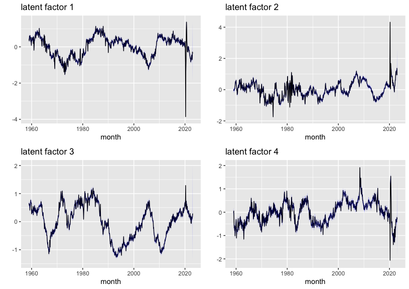
推定された隠れ時系列の細かい解釈は本記事の範囲外ですが、最初の四つの隠れ時系列はいずれもコロナ禍が始まった2020年1月当たりに急激な変化が見られたことを強調したいです。
続いては予測された時系列の全体の動きを確認しましょう。
ただ、変数が多いため、実質個人所得、民間雇用数、消費者物価指数、原油価格のみ可視化します。
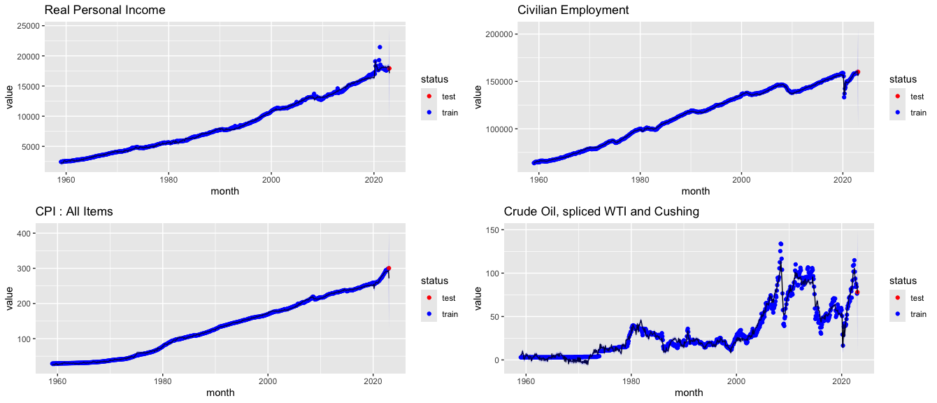
全体の傾向を表していると言えそうです!
精度確認
最後に検証データに対する予測精度を確認します。
評価指標として誤差率
$$|正解 - 予測結果|/正解$$
を利用します。
> m_fm_summary |>
     dplyr::filter(stringr::str_detect(variable, "value_predicted")) |>
     dplyr::bind_cols(ans = freq_df_with_id |>
                          dplyr::select(month, series, value)
     ) |>
     dplyr::mutate(
         month = as.Date(month),
         status = ifelse(month < as.Date("2023-01-01"), "train", "test"),
         error_ratio = abs((value - mean)/value),
         mean = round(mean, 2)
     ) |>
     dplyr::filter(status == "test") |>
     dplyr::select(series, value, mean, error_ratio) |>
     print(n = 200)
# A tibble: 108 × 4
    series                value       mean error_ratio
    <chr>                 <dbl>      <dbl>       <dbl>
  1 RPI               17921.      17125.       0.0444
  2 W875RX1           14745       14069.       0.0459
  3 DPCERA3M086SBEA     130.        121.       0.0689
  4 RETAILx          696982      599553.       0.140
  5 INDPRO              103.        100.       0.0264
  6 IPFPNSS             103.        101.       0.0156
  7 IPFINAL             104.        102.       0.0202
  8 IPCONGD             103.        101.       0.0255
  9 IPDCONGD            110.        105.       0.0533
 10 IPNCONGD            101.        100.       0.0114
 11 IPBUSEQ              96.9        95.6      0.0134
 12 IPMAT               103.         99.7      0.0317
 13 IPDMAT               96.2        94.3      0.0195
 14 IPNMAT               96.2        96.4      0.00283
 15 IPMANSICS           100.         98.5      0.0169
 16 IPB51222S            98.4       105.       0.0651
 17 IPFUELS              86.8        87.3      0.00568
 18 CUMFNS               77.7        76.7      0.0138
 19 CLF16OV          165832      161985.       0.0232
 20 CE16OV           160138      155846.       0.0268
 21 UNRATE                3.4         3.86     0.136
 22 UEMPMEAN             20.4        19.9      0.0257
 23 UEMPLT5            1946        2194.       0.127
 24 UEMP5TO14          1785        2033.       0.139
 25 UEMP15OV           2001        2046.       0.0223
 26 UEMP15T26           890         855.       0.0397
 27 UEMP27OV           1111        1187.       0.0688
 28 CLAIMSx          191750      270658.       0.412
 29 PAYEMS           155073      150270.       0.0310
 30 USGOOD            21514       21601.       0.00403
 31 CES1021000001       586.        635.       0.0841
 32 USCONS             7884        7720.       0.0208
 33 MANEMP            12999       13163.       0.0126
 34 DMANEMP            8102        8272.       0.0210
 35 NDMANEMP           4897        4903.       0.00131
 36 SRVPRD           133559      128320.       0.0392
 37 USTPU             28819       28166.       0.0226
 38 USWTRADE           6041        5957.       0.0139
 39 USTRADE           15483.      15460.       0.00147
 40 USFIRE             9114        8885.       0.0251
 41 USGOVT            22389       21990.       0.0178
 42 CES0600000007        40.8        40.4      0.00908
 43 AWOTMAN               3.8         3.72     0.0221
 44 AWHMAN               40.9        40.8      0.00265
 45 HOUST              1309        1365.       0.0425
 46 HOUSTNE             119         131.       0.0991
 47 HOUSTMW             123         180.       0.460
 48 HOUSTS              760         736.       0.0315
 49 HOUSTW              307         312.       0.0153
 50 PERMIT             1339        1454.       0.0861
 51 PERMITNE            106         132.       0.248
 52 PERMITMW            178         184.       0.0351
 53 PERMITS             762         807.       0.0587
 54 PERMITW             293         332.       0.134
 55 AMDMNOx          272257      248889.       0.0858
 56 ANDENOx           83875       80376.       0.0417
 57 AMDMUOx         1156999     1088231.       0.0594
 58 M1SL              19641       14980.       0.237
 59 M2SL              21267.      18552.       0.128
 60 M2REAL             7076.       6656.       0.0594
 61 BOGMBASE        5328400     4757822.       0.107
 62 TOTRESNS           3030.       2770.       0.0858
 63 NONBORRES       3014200     2734769.       0.0927
 64 BUSLOANS           2837.       2491.       0.122
 65 REALLN             5367.       4684        0.127
 66 FEDFUNDS              4.33        3.62     0.165
 67 CP3Mx                 4.61        4.01     0.131
 68 TB3MS                 4.54        3.73     0.178
 69 TB6MS                 4.67        3.82     0.182
 70 GS1                   4.69        4.1      0.126
 71 GS5                   3.64        3.55     0.0237
 72 GS10                  3.53        3.47     0.0183
 73 COMPAPFFx             0.28        0.37     0.323
 74 TB3SMFFM              0.21        0.13     0.382
 75 TB6SMFFM              0.34        0.26     0.221
 76 T1YFFM                0.36        0.47     0.303
 77 T5YFFM               -0.69        0        1.00
 78 T10YFFM              -0.8        -0.14     0.820
 79 AAAFFM                0.07        0.89    11.7
 80 EXSZUSx               0.924       0.93     0.00689
 81 EXJPUSx             130.        119        0.0877
 82 EXUSUKx               1.22        1.37     0.116
 83 EXCAUSx               1.34        1.33     0.0114
 84 WPSFD49207          257.        228.       0.114
 85 WPSFD49502          278.        244.       0.124
 86 WPSID61             264.        236.       0.108
 87 WPSID62             281.        257.       0.0846
 88 OILPRICEx            78.1        76.6      0.0194
 89 PPICMM              249.        242.       0.0303
 90 CPIAUCSL            301.        271.       0.0967
 91 CPIAPPSL            129.        125        0.0315
 92 CPITRNSL            263.        238.       0.0971
 93 CPIMEDSL            552.        511.       0.0740
 94 CUSR0000SAC         223.        204.       0.0831
 95 CUSR0000SAD         126.        121.       0.0406
 96 CUSR0000SAS         377.        341.       0.0957
 97 CPIULFSL            298.        271.       0.0902
 98 CUSR0000SA0L2       277.        252.       0.0877
 99 CUSR0000SA0L5       288.        261.       0.0940
100 PCEPI               126.        116.       0.0780
101 DDURRG3M086SBEA      96.9        97.6      0.00687
102 DNDGRG3M086SBEA     115.        106.       0.0754
103 DSERRG3M086SBEA     135.        123.       0.0906
104 CES0600000008        28.9        26.2      0.0945
105 CES2000000008        33.4        30        0.101
106 CES3000000008        25.8        23.5      0.0904
107 UMCSENTx             64.9        69.0      0.0629
108 INVEST             5515.       4762.       0.136
Moody’s Aaa Corporate Bond Minus FEDFUNDS(AAAFFM)のように大きく外れた変数もありますが、誤差率は全体的に低いです。All Employees: Nondurable goods(NDMANEMP)のように0.1%を達成した変数もあります。
全体の誤差率の平均も20%で、かなり信用できるモデルを構築できたのではないかと思います。
> m_fm_summary |>
     dplyr::filter(stringr::str_detect(variable, "value_predicted")) |>
     dplyr::bind_cols(ans = freq_df_with_id |>
                          dplyr::select(month, series, value)
     ) |>
     dplyr::mutate(
         month = as.Date(month),
         status = ifelse(month < as.Date("2023-01-01"), "train", "test"),
         error_ratio = abs((value - mean)/value),
         mean = round(mean, 2)
     ) |>
     dplyr::filter(status == "test") |>
     dplyr::pull(error_ratio) |>
     mean()
[1] 0.2052737959
結論
いかがでしたか?
ファクターモデルは高い予測性能を達成できるだけでなく、隠れ時系列に対する考察から手元のデータに対してより深い理解を得ることができます。
また、因果推論においては、欠損する処置状態のデータを補完するためにも利用できます。
興味ある方はBai and Ng(2021)を読んでみてください。
皆さんもぜひファクターモデルをご自身のデータ分析で活用してください!
参考資料
Bai, Jushan, and Serena Ng. "Matrix completion, counterfactuals, and factor analysis of missing data." Journal of the American Statistical Association 116.536 (2021): 1746-1763.
Bai, Jushan, and Peng Wang. "Identification and Bayesian estimation of dynamic factor models." Journal of Business & Economic Statistics 33.2 (2015): 221-240.