はじめに
本記事では、前回の記事の続きで
word2vecをベイズ機械学習の観点で一般化した指数族embedding(Rudolph et al. 2016)の一種をStanで実装する方法を紹介する。そして、実際に日本の衆議院の議事録の分析を行い、「アメリカ」と「アメリカ合衆国」と「米国」の意味の違い、及び「国際司法裁判所」に対する認識の変化などを可視化する。
内容が重複するので、word2vecの基本的な概念は省き、詳細は前回の記事と有名な論文(Mikolov et al. 2013など)を参考にしていただきたい。
今回のモデルの特殊性は、Rudolph and Blei(2018)を参考に、embeddingベクトルの時系列変化をランダムウォークでモデリングするところにある。ただし、Rudolph and Blei(2018)は全ての単語の変化の度合いの大きさに同一のパラメータを付与するのに対し、本記事のモデルでは全ての単語のそれぞれの時系列変化の大きさのパラメータを付与する。
モデル説明
事前分布
本記事で利用するモデルは、構造的には潜在変数がランダムウォークに従って変化するベイズモデルに近い。パラメータ群が従う事前分布は具体的には下記の通りである:
\begin{align}
&embedding\_sigma_{word = w} \sim gamma(0.1, 0.1)\\\\

&word\_context \sim normal(0,1) \\\\

&word\_embedding_{t = 1, word = w} \sim normal(0, 1) \\\\

&word\_embedding_{t = t + 1, word = w} \sim normal(word\_embedding_{t = t, word = w}, \space embedding\_sigma_{word = w}^2)

\end{align}
要するに、contextベクトルは時間と共に変化しないが、embeddingベクトルは時間と共にランダムウォークに従って変化する。また、embeddingベクトルの変化の大きさは単語によって異なる。
contextベクトルを一定とする理由は、Rudolph and Blei(2018)が指摘したように、時間と共に変化するembeddingベクトルが同じで比較可能な意味空間(semantic space)に存在することを担保するためである。
尤度関数
次に、尤度関数の構造を紹介する。本物フラグとは、ネガティブサンプリング時にサンダムに抽出したデタラメのデータなのか、それとも本当のデータに実在するデータなのかを示すフラグである。
本物フラグ \sim bernoulli(logit(word\_embedding_{t = t, word = w} * \Sigma_{context}word\_context))
上記の数式の構造から分かるように、モデルは判断の目標となる単語が出現した時間(年度など)からembeddingベクトルを引っ張ってきて、その単語の周辺の単語のcontextベクトルの和と内積を取ることで、本物かデタラメかを判断する。
Stanのコード
本記事の分析で利用するStanのコードは、上記のベイズ機械学習モデル自体を実装する内容の他に、検証データに対して予測を行う処理とF1 scoreの事後分布を計算する方法も含まれている。
機械学習でよく利用される評価指標の事後分布の推定に関する文献は不勉強でまだ確認していないが、パラメータの不確実性から波及された評価指標の振れと解釈できると思われる。
機械学習の評価指標の事後分布の推定についてはそもそもどんな研究をされているかも含めて別記事で紹介する予定である。
functions {
  real partial_sum_lpmf(
    array[,] int big_matrix,
    int start, int end,

    array[,] vector word_embedding,
    array[] vector word_context
  ){
    vector[end - start + 1] lambda;
    int count = 1;
    for (i in start:end){
      lambda[count] = word_embedding[big_matrix[count, 2], big_matrix[count, 1]] ' *
      (
        word_context[big_matrix[count, 3]] + word_context[big_matrix[count, 4]] +
        word_context[big_matrix[count, 5]] + word_context[big_matrix[count, 6]] +
        word_context[big_matrix[count, 7]] + word_context[big_matrix[count, 8]] +
        word_context[big_matrix[count, 9]] + word_context[big_matrix[count, 10]] +
        word_context[big_matrix[count, 11]] + word_context[big_matrix[count, 12]]
      );
      count += 1;
    }
    return (
      bernoulli_logit_lupmf(big_matrix[, 13] | lambda)
    );
  }
}

data {
  int<lower=1> N; //学習データ数
  int<lower=1> K; //embedding次元数
  int<lower=1> word_type; //単語数
  int<lower=1> year_type; //年の数

  //学習データ
  array[N] int<lower=1,upper=word_type> word;
  array[N] int<lower=1,upper=year_type> year;
  array[N] int<lower=1,upper=word_type> word_before_1;
  array[N] int<lower=1,upper=word_type> word_after_1;
  array[N] int<lower=1,upper=word_type> word_before_2;
  array[N] int<lower=1,upper=word_type> word_after_2;
  array[N] int<lower=1,upper=word_type> word_before_3;
  array[N] int<lower=1,upper=word_type> word_after_3;
  array[N] int<lower=1,upper=word_type> word_before_4;
  array[N] int<lower=1,upper=word_type> word_after_4;
  array[N] int<lower=1,upper=word_type> word_before_5;
  array[N] int<lower=1,upper=word_type> word_after_5;
  array[N] int<lower=0,upper=1> result;

  int<lower=0> val_N; //検証データ数
  //検証データ
  array[val_N] int<lower=1,upper=word_type> val_word;
  array[val_N] int<lower=1,upper=year_type> val_year;
  array[val_N] int<lower=1,upper=word_type> val_word_before_1;
  array[val_N] int<lower=1,upper=word_type> val_word_after_1;
  array[val_N] int<lower=1,upper=word_type> val_word_before_2;
  array[val_N] int<lower=1,upper=word_type> val_word_after_2;
  array[val_N] int<lower=1,upper=word_type> val_word_before_3;
  array[val_N] int<lower=1,upper=word_type> val_word_after_3;
  array[val_N] int<lower=1,upper=word_type> val_word_before_4;
  array[val_N] int<lower=1,upper=word_type> val_word_after_4;
  array[val_N] int<lower=1,upper=word_type> val_word_before_5;
  array[val_N] int<lower=1,upper=word_type> val_word_after_5;
  array[val_N] int<lower=0,upper=1> val_result;
}
transformed data {
  // embeddingベクトルとcontextベクトル以外で尤度関数の計算で利用するデータをまとめる
  array[N, 13] int big_matrix;
  big_matrix[,1] = word;
  big_matrix[,2] = year;
  big_matrix[,3] = word_before_1;
  big_matrix[,4] = word_after_1;
  big_matrix[,5] = word_before_2;
  big_matrix[,6] = word_after_2;
  big_matrix[,7] = word_before_3;
  big_matrix[,8] = word_after_3;
  big_matrix[,9] = word_before_4;
  big_matrix[,10] = word_after_4;
  big_matrix[,11] = word_before_5;
  big_matrix[,12] = word_after_5;
  big_matrix[,13] = result;
}
parameters {
  vector<lower=0>[word_type] embedding_sigma;
  array[year_type, word_type] vector[K] word_embedding;
  array[word_type] vector[K] word_context;
}
model {
  target += gamma_lupdf(embedding_sigma | 0.1, 0.1);

  for (p in 1:word_type){
    target += normal_lupdf(word_embedding[1, p] | 0, 1);
    for (t in 2:year_type){
      target += normal_lupdf(word_embedding[t, p] | word_embedding[t - 1, p], embedding_sigma[p]^2);
    }
    target += normal_lupdf(word_context[p] | 0, 1);
  }

  int grainsize = 1;

  target += reduce_sum(
    partial_sum_lupmf, big_matrix, grainsize,

    word_embedding,
    word_context
  );
}
generated quantities {
  array[val_N] int predicted;
  real F1_score;
  for (n in 1:val_N){
    predicted[n] = bernoulli_logit_rng(
      word_embedding[val_year[n], val_word[n]] ' *
      (
        word_context[val_word_before_1[n]] + word_context[val_word_after_1[n]] +
        word_context[val_word_before_2[n]] + word_context[val_word_after_2[n]] +
        word_context[val_word_before_3[n]] + word_context[val_word_after_3[n]] +
        word_context[val_word_before_4[n]] + word_context[val_word_after_4[n]] +
        word_context[val_word_before_5[n]] + word_context[val_word_after_5[n]]
      )
    );
  }
  {
    int TP = 0;
    int FP = 0;
    int FN = 0;
    for (n in 1:val_N){
      if (val_result[n] == 1 && predicted[n] == 1){
        TP += 1;
      }
      else if (val_result[n] == 0 && predicted[n] == 1){
        FP += 1;
      }
      else if (val_result[n] == 1 && predicted[n] == 0){
        FN += 1;
      }
    }
    F1_score = (2 * TP) * 1.0/(2 * TP + FP + FN);
  }
}
分析
前処理
本記事では、下記のサイトを参考に、衆議院の外務委員会の議事録を上記の手法で分析し、日本の国会議員の言説の変化を可視化する。
ただし、本記事の目的はアルゴリズムの動作確認にあるため、比較政治学と国際政治学の基準を満たすような前処理の厳密さはないことはあらかじめ強調しておきたい。ビジネスの世界でもアカデミアの世界でもそうだが、アイデアがしっかり動くことを確認してから、中身をブラッシュアップするという手順を踏めば、プロジェクト・論文執筆はスムーズに進む。
若干話しが逸れるが、筆者も最近業務でテキストアズデータの手法を用いて深く考えすぎずにとりあえず手元のデータで分析を回してビジネス側の方に見せたら、「なるほど!こんな仕組みのモデルだよね!だったらXとYもZが理由で変数に入れた方がいいよ、私がSQLを書くよ!」などのアクショナブルで素晴らしいフィードバックをたくさんいただいた。
最初から完璧な分析結果を求めすぎず、非定量分析者がドメイン知識でコメントできるレベルの暫定的な成果物で十分である。まず動くものを作れば協力者たちとのコミュニケーションも取りやすくなり、みんなの力を合わせてもっといいものが出来上がる。
では、前処理の話に戻ると、まずは、大前提となるmecabの処理フローを関数化する。
mecabbing <- function(text){
  this_review <- stringr::str_replace_all(text, "[^一-龠ぁ-んーァ-ヶーa-zA-Z]", " ")
  mecab_output <- unlist(RMeCab::RMeCabC(this_review, 1))
  mecab_combined <- stringr::str_c(mecab_output[which(names(mecab_output) == "名詞")], collapse = " ")
  return(mecab_combined)
}
次に、上記のQuantedaのサイトを参考に必要なデータの抽出を行う
# データのダウンロード
full_corp <- quanteda.corpora::download("data_corpus_foreignaffairscommittee") |>
  quanteda::corpus_subset(speaker != "")

# 肩書きを含む人名の抽出
capacity_full <- full_corp |>
  stringr::str_sub(1, 20) |>
  stringr::str_replace_all("\\s+.+|\n", "") |> # 冒頭の名前部分の取り出し
  stringr::str_replace( "^.+[参事|政府特別補佐人|内閣官房|会計検査院|最高裁判所長官代理者|主査|議員|副?大臣|副?議長|委員|参考人|分科員|公述人|]君((.+))?$", "\\1")

# 肩書きの抽出
capacity <- full_corp |>
  stringr::str_sub(1, 20) |>
  stringr::str_replace_all("\\s+.+|\n", "") |> # 冒頭の名前部分の取り出し
  stringr::str_replace( "^.+?(参事|政府特別補佐人|内閣官房|会計検査院|最高裁判所長官代理者|主査|議員|副?大臣|副?議長|委員|参考人|分科員|公述人|君((.+))?$)", "\\1") |>  # 冒頭の○から,名前部分までを消去
  stringr::str_replace("(.+)", "") |>
  stringr::str_replace("^○.+", "Other")

# 年の抽出
record_year <- docvars(full_corp, "date") |>
  lubridate::year() |>
  as.numeric()
続いては、まずfurrrによるmecabの並列処理の準備をして、分析用のデータフレイム(tibble)を作成する。
# 並列処理の準備
future::plan(future::multisession, workers = 16)

sub_corp_df <- tibble::tibble(
  capacity_full = capacity_full,
  capacity = capacity,
  record_year = record_year,
  # テキストデータ形式をquantedaからbase Rのcharacter型に変換する
  text = full_corp |>
    as.list() |>
    unlist()
) |>
  dplyr::filter(dplyr::between(record_year, 1991, 2017)) |>
  dplyr::filter(capacity %in% c("委員", "大臣", "副大臣")) |>
  # 発言の冒頭の名前と肩書きを削除
  dplyr::mutate(
    text = stringr::str_remove_all(text, stringr::fixed(capacity_full))
  ) |>
  dplyr::mutate(text_mecabbed = furrr::future_map_chr(text, ~ mecabbing(.x))) |>
  dplyr::mutate(
    text_id = dplyr::row_number()
  )
次のステップとして、quantedaの機能を使って使われすぎた単語と使われなさすぎた単語を削除して、実際に分析で利用する単語をまとめた単語のマスターテーブルを作成する。
sub_corp_use_tokens <- sub_corp_df |>
  dplyr::pull(text_mecabbed) |>
  quanteda::phrase() |>
  quanteda::tokens() |>
  quanteda::tokens_remove("の") |>
  quanteda::dfm() |>
  quanteda::dfm_trim(min_termfreq = 100, max_termfreq = 30000) |>
  colnames()

word_master <- tibble::tibble(
  word = sub_corp_use_tokens
) |>
  dplyr::arrange(word) |>
  dplyr::mutate(
    word_id = dplyr::row_number()
  )
ここで、tidyrの機能を活用して、一レコード一文の形式のデータフレイムを一レコード一単語の形式に変換する。
sub_corp_long_df <- sub_corp_df |>
  dplyr::select(text_id, record_year, text_mecabbed) |>
  dplyr::mutate(
    word = text_mecabbed |>
      quanteda::phrase() |>
      quanteda::tokens() |>
      quanteda::tokens_remove("の") |>
      as.list()
  ) |>
  tidyr::unnest_longer(word) |>
  dplyr::filter(word %in% word_master$word) |>
  dplyr::select(text_id, record_year, word) |>
  dplyr::group_by(text_id, record_year) |>
  # 周囲のcontextを抽出するためにposition idを付与する
  dplyr::mutate(position_id = dplyr::row_number()) |>
  dplyr::ungroup() |>
  dplyr::left_join(word_master, by = "word")
具体的な処理結果は下記の通りである:
> sub_corp_long_df
# A tibble: 3,099,254 × 5
   text_id record_year word     position_id word_id
     <int>       <dbl> <chr>          <int>   <int>
 1       1        1991 十一月             1     997
 2       1        1991 五                 2     611
 3       1        1991 外務               3    1269
 4       1        1991 あいさつ           4       2
 5       1        1991 機会               5    2032
 6       1        1991 歴史               6    2072
 7       1        1991 国際               7    1196
 8       1        1991 社会               8    2406
 9       1        1991 冷戦               9     892
10       1        1991 対話              10    1419
# ℹ 3,099,244 more rows
# ℹ Use `print(n = ...)` to see more rows
次に、単語の前後の五つの単語を持ってくる処理を行う。
sub_corp_long_df_lag_correct <- sub_corp_long_df |>
  dplyr::left_join(
    sub_corp_long_df |>
      dplyr::mutate(
        position_id = position_id - 1
      ) |>
      dplyr::rename("word_id_after_1" = word_id) |>
      dplyr::select(text_id, position_id, word_id_after_1),
    by = c("text_id" = "text_id", "position_id" = "position_id")
  ) |>
  dplyr::left_join(
    sub_corp_long_df |>
      dplyr::mutate(
        position_id = position_id - 2
      ) |>
      dplyr::rename("word_id_after_2" = word_id) |>
      dplyr::select(text_id, position_id, word_id_after_2),
    by = c("text_id" = "text_id", "position_id" = "position_id")
  ) |>
  dplyr::left_join(
    sub_corp_long_df |>
      dplyr::mutate(
        position_id = position_id - 3
      ) |>
      dplyr::rename("word_id_after_3" = word_id) |>
      dplyr::select(text_id, position_id, word_id_after_3),
    by = c("text_id" = "text_id", "position_id" = "position_id")
  ) |>
  dplyr::left_join(
    sub_corp_long_df |>
      dplyr::mutate(
        position_id = position_id - 4
      ) |>
      dplyr::rename("word_id_after_4" = word_id) |>
      dplyr::select(text_id, position_id, word_id_after_4),
    by = c("text_id" = "text_id", "position_id" = "position_id")
  ) |>
  dplyr::left_join(
    sub_corp_long_df |>
      dplyr::mutate(
        position_id = position_id - 5
      ) |>
      dplyr::rename("word_id_after_5" = word_id) |>
      dplyr::select(text_id, position_id, word_id_after_5),
    by = c("text_id" = "text_id", "position_id" = "position_id")
  ) |>
  dplyr::left_join(
    sub_corp_long_df |>
      dplyr::mutate(
        position_id = position_id + 1
      ) |>
      dplyr::rename("word_id_before_1" = word_id) |>
      dplyr::select(text_id, position_id, word_id_before_1),
    by = c("text_id" = "text_id", "position_id" = "position_id")
  ) |>
  dplyr::left_join(
    sub_corp_long_df |>
      dplyr::mutate(
        position_id = position_id + 2
      ) |>
      dplyr::rename("word_id_before_2" = word_id) |>
      dplyr::select(text_id, position_id, word_id_before_2),
    by = c("text_id" = "text_id", "position_id" = "position_id")
  ) |>
  dplyr::left_join(
    sub_corp_long_df |>
      dplyr::mutate(
        position_id = position_id + 3
      ) |>
      dplyr::rename("word_id_before_3" = word_id) |>
      dplyr::select(text_id, position_id, word_id_before_3),
    by = c("text_id" = "text_id", "position_id" = "position_id")
  ) |>
  dplyr::left_join(
    sub_corp_long_df |>
      dplyr::mutate(
        position_id = position_id + 4
      ) |>
      dplyr::rename("word_id_before_4" = word_id) |>
      dplyr::select(text_id, position_id, word_id_before_4),
    by = c("text_id" = "text_id", "position_id" = "position_id")
  ) |>
  dplyr::left_join(
    sub_corp_long_df |>
      dplyr::mutate(
        position_id = position_id + 5
      ) |>
      dplyr::rename("word_id_before_5" = word_id) |>
      dplyr::select(text_id, position_id, word_id_before_5),
    by = c("text_id" = "text_id", "position_id" = "position_id")
  ) |>
  tidyr::drop_na() |>
  dplyr::select(!word) |>
  # 本物フラグを作成
  dplyr::mutate(
    ans = 1
  )
最後に、ネガティブサンプリングを実行し、年IDを作成する。もともと全ての年についてIDを付与したかったが、計算時間の問題を考慮して、本記事ではやむをえず五年単位でIDを付与する。
set.seed(12345)

neg_sample <- sample(sub_corp_long_df_lag_correct$word_id, length(sub_corp_long_df_lag_correct$word_id), replace = FALSE)

longer_df_with_id_neg <- sub_corp_long_df_lag_correct |>
  dplyr::mutate(word_id = neg_sample) |>
  dplyr::mutate(ans = 0)

sub_corp_long_df_lag_correct_and_neg <- sub_corp_long_df_lag_correct |>
  dplyr::bind_rows(
    longer_df_with_id_neg
  ) |>
  dplyr::mutate(
    year_group = dplyr::case_when(
      dplyr::between(record_year, 1991, 1995) ~ 1,
      dplyr::between(record_year, 1996, 2000) ~ 2,
      dplyr::between(record_year, 2001, 2005) ~ 3,
      dplyr::between(record_year, 2006, 2010) ~ 4,
      dplyr::between(record_year, 2011, 2015) ~ 5,
      TRUE ~ 6
    )
  )
Stanに実際にデータを入れる前に、学習データと検証データに分けてlistに整理し、さらにstanのコードのコンパイルも行う。
set.seed(12345)

full_id <- sample(1:nrow(sub_corp_long_df_lag_correct_and_neg), nrow(sub_corp_long_df_lag_correct_and_neg) * 1, replace = FALSE)
test_id <- full_id[1:5000]

train_id <- full_id[5001:length(full_id)]

data_list <- list(
  N = nrow(sub_corp_long_df_lag_correct_and_neg[train_id,]),
  K = 20,
  word_type = nrow(word_master),
  year_type = length(unique(sub_corp_long_df_lag_correct_and_neg$year_group)),
  word = sub_corp_long_df_lag_correct_and_neg$word_id[train_id],
  year = sub_corp_long_df_lag_correct_and_neg$year_group[train_id],
  word_before_1 = sub_corp_long_df_lag_correct_and_neg$word_id_before_1[train_id],
  word_after_1 = sub_corp_long_df_lag_correct_and_neg$word_id_after_1[train_id],
  word_before_2 = sub_corp_long_df_lag_correct_and_neg$word_id_before_2[train_id],
  word_after_2 = sub_corp_long_df_lag_correct_and_neg$word_id_after_2[train_id],
  word_before_3 = sub_corp_long_df_lag_correct_and_neg$word_id_before_3[train_id],
  word_after_3 = sub_corp_long_df_lag_correct_and_neg$word_id_after_3[train_id],
  word_before_4 = sub_corp_long_df_lag_correct_and_neg$word_id_before_4[train_id],
  word_after_4 = sub_corp_long_df_lag_correct_and_neg$word_id_after_4[train_id],
  word_before_5 = sub_corp_long_df_lag_correct_and_neg$word_id_before_5[train_id],
  word_after_5 = sub_corp_long_df_lag_correct_and_neg$word_id_after_5[train_id],
  result = sub_corp_long_df_lag_correct_and_neg$ans[train_id],

  val_N = length(test_id),
  val_word = sub_corp_long_df_lag_correct_and_neg$word_id[test_id],
  val_year = sub_corp_long_df_lag_correct_and_neg$year_group[test_id],
  val_word_before_1 = sub_corp_long_df_lag_correct_and_neg$word_id_before_1[test_id],
  val_word_after_1 = sub_corp_long_df_lag_correct_and_neg$word_id_after_1[test_id],
  val_word_before_2 = sub_corp_long_df_lag_correct_and_neg$word_id_before_2[test_id],
  val_word_after_2 = sub_corp_long_df_lag_correct_and_neg$word_id_after_2[test_id],
  val_word_before_3 = sub_corp_long_df_lag_correct_and_neg$word_id_before_3[test_id],
  val_word_after_3 = sub_corp_long_df_lag_correct_and_neg$word_id_after_3[test_id],
  val_word_before_4 = sub_corp_long_df_lag_correct_and_neg$word_id_before_4[test_id],
  val_word_after_4 = sub_corp_long_df_lag_correct_and_neg$word_id_after_4[test_id],
  val_word_before_5 = sub_corp_long_df_lag_correct_and_neg$word_id_before_5[test_id],
  val_word_after_5 = sub_corp_long_df_lag_correct_and_neg$word_id_after_5[test_id],
  val_result = sub_corp_long_df_lag_correct_and_neg$ans[test_id]
)

m_init <- cmdstanr::cmdstan_model("dyn_emb.stan",
                                  cpp_options = list(
                                    stan_threads = TRUE
                                  )
)
モデル推定
さて、ここで実際のモデルの推定に入るが、ものすごく時間がかかるため、再現したい方はもし可能ならOpencl経由でGPUを使ってみてください。M1 Macには対応していないようなので、筆者のように少し待つか、クラウドサービスを用いた分析環境を検討してください。
> m_estimate <- m_init$variational(
     seed = 12345,
     threads = 6,
     iter = 50000,
     data = data_list
 )
------------------------------------------------------------
EXPERIMENTAL ALGORITHM:
  This procedure has not been thoroughly tested and may be unstable
  or buggy. The interface is subject to change.
------------------------------------------------------------
Gradient evaluation took 7.82436 seconds
1000 transitions using 10 leapfrog steps per transition would take 78243.6 seconds.
Adjust your expectations accordingly!
Begin eta adaptation.
Iteration:   1 / 250 [  0%]  (Adaptation)
Iteration:  50 / 250 [ 20%]  (Adaptation)
Iteration: 100 / 250 [ 40%]  (Adaptation)
Iteration: 150 / 250 [ 60%]  (Adaptation)
Iteration: 200 / 250 [ 80%]  (Adaptation)
Iteration: 250 / 250 [100%]  (Adaptation)
Success! Found best value [eta = 0.1].
Begin stochastic gradient ascent.
  iter             ELBO   delta_ELBO_mean   delta_ELBO_med   notes
   100   -753139313.982             1.000            1.000
   200   -653411538.557             0.576            1.000
   300    -61853447.001             3.572            1.000
   400    -22863342.956             3.105            1.705
   500    -10794778.330             2.708            1.118
   600     -5763861.305             2.402            1.118
   700     -4377611.199             2.104            1.000
   800     -3594931.914             1.868            1.000
   900     -3261148.443             1.672            0.873
  1000     -3105653.178             1.510            0.873
  1100     -2976329.907             1.377            0.317   MAY BE DIVERGING... INSPECT ELBO
  1200     -2914750.721             1.264            0.317   MAY BE DIVERGING... INSPECT ELBO
  1300     -2878920.212             1.167            0.218   MAY BE DIVERGING... INSPECT ELBO
  1400     -2841154.722             1.085            0.218   MAY BE DIVERGING... INSPECT ELBO
  1500     -2820317.186             1.013            0.153   MAY BE DIVERGING... INSPECT ELBO
  1600     -2805134.420             0.950            0.153   MAY BE DIVERGING... INSPECT ELBO
  1700     -2793821.362             0.895            0.102   MAY BE DIVERGING... INSPECT ELBO
  1800     -2785226.804             0.845            0.102   MAY BE DIVERGING... INSPECT ELBO
  1900     -2777701.626             0.801            0.050   MAY BE DIVERGING... INSPECT ELBO
  2000     -2772061.428             0.761            0.050   MAY BE DIVERGING... INSPECT ELBO
  2100     -2767432.422             0.725            0.043   MAY BE DIVERGING... INSPECT ELBO
  2200     -2763751.392             0.692            0.043   MAY BE DIVERGING... INSPECT ELBO
  2300     -2760474.745             0.662            0.021   MAY BE DIVERGING... INSPECT ELBO
  2400     -2757840.731             0.634            0.021   MAY BE DIVERGING... INSPECT ELBO
  2500     -2755665.109             0.609            0.013   MAY BE DIVERGING... INSPECT ELBO
  2600     -2753664.624             0.585            0.013   MAY BE DIVERGING... INSPECT ELBO
  2700     -2752144.973             0.564            0.012   MAY BE DIVERGING... INSPECT ELBO
  2800     -2750702.229             0.544            0.012   MAY BE DIVERGING... INSPECT ELBO
  2900     -2749365.397             0.525            0.007   MEDIAN ELBO CONVERGED   MAY BE DIVERGING... INSPECT ELBO
Drawing a sample of size 1000 from the approximate posterior...
COMPLETED.
Finished in  27050.3 seconds.
かなり時間がかかった。
まずは結果のサマリーを保存する。
m_summary <- m_estimate$summary()
評価指標の事後分布
次に、評価指標のF1 scoreの事後分布を確認する。
m_estimate$draws("F1_score") |>
  tibble::as_tibble() |>
  dplyr::mutate(F1_score = as.numeric(F1_score)) |>
  ggplot2::ggplot() +
  ggplot2::geom_density(ggplot2::aes(x = F1_score),
                        fill = ggplot2::alpha("blue", 0.3)) +
  ggplot2::ggtitle("ベイズ動的word2vecのF1 scoreの事後分布") +
  ggplot2::theme_gray(base_family = "HiraKakuPro-W3")
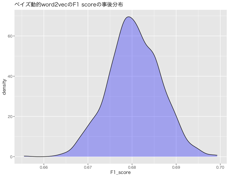
このように、F1 scoreの事後分布は0.68付近に集まっており、かつ0.7と0.66の範囲をはみ出す確率は低いことを視覚的に確認できる。
よって、ある程度精度が出ているものの、このモデルは本物かデタラメかを判定する性能が特に優れているとはいえない。計算時間のためにembeddingの次元数を絞ったのが理由だと思われる。
ただ、ここで強調しておきたいのは、分類や予測の良さの測定に最適化された機械学習の評価指標の良し悪しは、モデルが抽出したQOI(quantities of interest)の質を含意しない。
単語の意味の変化
ここからは本モデルの特徴である単語の意味の変化の分析を行う。
変化の大きさ
まずは、前述のように、本モデルはRudolph and Blei(2018)と違って全ての単語にそれぞれの経時的な変化の大きさのパラメータを設定しているので、まずは経時的な変化が大きい単語から確認する。
> word_master |>
     dplyr::bind_cols(
         e = m_summary |>
             dplyr::filter(stringr::str_detect(variable, "embedding_sigma")) |>
             dplyr::pull(mean)
     ) |>
     dplyr::arrange(-e) |>
     print(n = 20)
# A tibble: 3,171 × 3
   word           word_id     e
   <chr>            <int> <dbl>
 1 着席              2378  1.53
 2 社会民主党        2408  1.42
 3 亮                 623  1.26
 4 平沢              1492  1.25
 5 拍手              1705  1.16
 6 政                1790  1.14
 7 高野              3164  1.11
 8 ここら             139  1.10
 9 太郎              1320  1.09
10 丸谷               567  1.09
11 篠原              2485  1.09
12 阿南              3066  1.08
13 東西              1968  1.08
14 赤嶺              2857  1.08
15 維新              2531  1.07
16 いか                35  1.06
17 ギョーザ           119  1.06
18 メドベージェフ     416  1.05
19 薮                2635  1.05
20 首藤              3150  1.04
# ℹ 3,151 more rows
# ℹ Use `print(n = ...)` to see more rows
次に、経時的な変化が少ない単語は下記の通りである。
> word_master |>
     dplyr::bind_cols(
         e = m_summary |>
             dplyr::filter(stringr::str_detect(variable, "embedding_sigma")) |>
             dplyr::pull(mean)
     ) |>
     dplyr::arrange(e) |>
     print(n = 20)
# A tibble: 3,171 × 3
   word   word_id     e
   <chr>    <int> <dbl>
 1 今         644 0.239
 2 一         458 0.253
 3 方        1836 0.272
 4 等        2472 0.276
 5 必要      1588 0.278
 6 意味      1616 0.281
 7 何         718 0.283
 8 とき       278 0.285
 9 政府      1794 0.285
10 関係      3050 0.286
11 状況      2241 0.288
12 先         791 0.289
13 人         624 0.291
14 ここ       138 0.294
15 ところ     280 0.295
16 一つ       459 0.296
17 点        2197 0.298
18 間        3046 0.299
19 年        1495 0.302
20 我が国    1648 0.304
# ℹ 3,151 more rows
# ℹ Use `print(n = ...)` to see more rows
上記の結果からも分かるように、経時的な変化が特に大きいのは、「東西(陣営・冷戦)」や「メドベージェフ」などの人名や時代背景に関連する単語であるのに対し、「関係」、「政府」のような一般的な用語は変化が少ない。これは我々の定性的な認識と一致している。
変化の可視化
ここでは、単語の意味の変化自体の可視化を行う。そのために、まずパラメータをlist型に整形する処理をする。
word_embedding_df <- m_summary |>
  dplyr::filter(stringr::str_detect(variable, "word_embedding")) |>
  # word_embeddingのインデックスは[年ID, 単語ID, embedding次元]なので、
  # 年ID, 単語ID, embedding次元を取り出して別々のカラムを作る
  dplyr::mutate(
    index = purrr::map(variable, ~ as.numeric(stringr::str_split_fixed(.x, "\\[|\\]|,", 5)[1,2:4]))
  ) |>
  tidyr::unnest_wider(index, names_sep = "_")

word_embedding_list <- list()

for (i in 1:6){
  word_embedding_list[[i]] <- word_embedding_df |>
    # index_1が年ID
    dplyr::filter(index_1 == i) |>
    dplyr::pull(mean) |>
    matrix(ncol = 20)
}
そして、コサイン類似度を取得する関数と各時期のコサイン類似度を降順で単語を並べたデータフレイムにまとめる関数を作成する。
get_cos_sim <- function(time, word_id, word_embedding_list){
  cos_sim <- c()
  for (i in 1:nrow(word_master)){
    cos_sim[i] <- (word_embedding_list[[time]][word_id,] %*% word_embedding_list[[time]][i,])/sqrt(sum(word_embedding_list[[time]][word_id,]^2) * sum(word_embedding_list[[time]][i,]^2))
  }
  return(cos_sim)
}

get_cos_sim_df <- function(word_id, word_embedding_list, word_master){
  cos_sim_df <- word_master |>
    dplyr::bind_cols(e = get_cos_sim(1, word_id, word_embedding_list)) |>
    dplyr::arrange(-e) |>
    dplyr::select(word) |>
    dplyr::bind_cols(
      word_master |>
        dplyr::bind_cols(e = get_cos_sim(2, word_id, word_embedding_list)) |>
        dplyr::arrange(-e) |>
        dplyr::select(word)
    ) |>
    dplyr::bind_cols(
      word_master |>
        dplyr::bind_cols(e = get_cos_sim(3, word_id, word_embedding_list)) |>
        dplyr::arrange(-e) |>
        dplyr::select(word)
    ) |>
    dplyr::bind_cols(
      word_master |>
        dplyr::bind_cols(e = get_cos_sim(4, word_id, word_embedding_list)) |>
        dplyr::arrange(-e) |>
        dplyr::select(word)
    ) |>
    dplyr::bind_cols(
      word_master |>
        dplyr::bind_cols(e = get_cos_sim(5, word_id, word_embedding_list)) |>
        dplyr::arrange(-e) |>
        dplyr::select(word)
    ) |>
    dplyr::bind_cols(
      word_master |>
        dplyr::bind_cols(e = get_cos_sim(6, word_id, word_embedding_list)) |>
        dplyr::arrange(-e) |>
        dplyr::select(word)
    )


  colnames(cos_sim_df) <- c("1991~1995", "1996~2000", "2001~2005", "2006~2010", "2010~2015", "2016~2017")

  return(cos_sim_df)
}
さて、ここでいよいよ単語の変化を可視化するところに入る。まずは概念系の「人権」という単語とコサイン類似度の高い、つまり同じ文脈で語られがちな単語の変化から確認する:
> get_cos_sim_df(633, word_embedding_list, word_master)
New names:
• `word` -> `word...1`
• `word` -> `word...2`
New names:
• `word` -> `word...3`
New names:
• `word` -> `word...4`
New names:
• `word` -> `word...5`
New names:
• `word` -> `word...6`
# A tibble: 3,171 × 6
   `1991~1995` `1996~2000` `2001~2005` `2006~2010` `2010~2015` `2016~2017`
   <chr>       <chr>       <chr>       <chr>       <chr>       <chr>
 1 人権        人権        人権        人権        人権        人権
 2 人種        侵害        侵害        侵害        普遍        招致
 3 子ども      憲章        差別        普遍        舞台        差別
 4 子供        普遍        普遍        あらわれ    女性        腐敗
 5 社会        社会        人種        規約        尊重        規約
 6 普遍        児童        社会        挑戦        決議        舞台
 7 差別        先頭        主権        民主        挑戦        理事
 8 精神        撲滅        精神        協調        規約        勧告
 9 侵害        人種        認知        毅然        国連        決議
10 生存        主義        権利        社会        批准        支配
# ℹ 3,161 more rows
# ℹ Use `print(n = ...)` to see more rows
ここから分かるのは、少なくとも衆議院の外務委員会の委員、大臣、副大臣の中で、人権は1990年代は児童と共に語られていたが、2000年代以降では児童と共に語られることが少なくなった。これは日本ないし国際社会が重視する人権の種類の変化を可視化できたといえよう。
二つ目の概念系の単語として、「正義」とコサイン類似度の高い単語の変化を見てみよう:
> get_cos_sim_df(2061, word_embedding_list, word_master)
New names:
• `word` -> `word...1`
• `word` -> `word...2`
New names:
• `word` -> `word...3`
New names:
• `word` -> `word...4`
New names:
• `word` -> `word...5`
New names:
• `word` -> `word...6`
# A tibble: 3,171 × 6
   `1991~1995` `1996~2000` `2001~2005` `2006~2010`    `2010~2015`    `2016~2017`
   <chr>       <chr>       <chr>       <chr>          <chr>          <chr>
 1 正義        正義        正義        正義           正義           正義
 2 国家        武装        統治        海部           国際司法裁判所 国際司法裁判所
 3 主義        国家        主義        国際司法裁判所 宣言           談話
 4 実力        主義        海部        統治           村山           宣言
 5 憲法        和解        侵略        主義           福田           用語
 6 統治        哲学        憲法        国家           内政           侵略
 7 独立        施政        戦争        ライン         主義           秩序
 8 平和        集団        国家        人種           哲学           福田
 9 主権        独立        集団        侵略           戦争           樹立
10 普遍        ソ連邦      勢力        秩序           精神           村山
# ℹ 3,161 more rows
# ℹ Use `print(n = ...)` to see more rows
かなり明確だが、2006年から「国際司法裁判所」と共に語られるようになった。これの理由はすぐには思いつかないので、「国際司法裁判所」と類似している単語の変化を確認する:
> get_cos_sim_df(1197, word_embedding_list, word_master)
New names:
• `word` -> `word...1`
• `word` -> `word...2`
New names:
• `word` -> `word...3`
New names:
• `word` -> `word...4`
New names:
• `word` -> `word...5`
New names:
• `word` -> `word...6`
# A tibble: 3,171 × 6
   `1991~1995`    `1996~2000`    `2001~2005`    `2006~2010`    `2010~2015`    `2016~2017`
   <chr>          <chr>          <chr>          <chr>          <chr>          <chr>
 1 国際司法裁判所 国際司法裁判所 国際司法裁判所 国際司法裁判所 国際司法裁判所 国際司法裁判所
 2 証拠           違法           画定           画定           正義           宮澤
 3 違法           文             違法           固有           内政           論理
 4 発見           違反           共謀           正義           論理           正義
 5 処分           証拠           固有           大陸棚         反論           内政
 6 客観           行為           領有           領有           云             スタンス
 7 有無           声明           手順           表示           我             コンセンサス
 8 違反           即時           声明           捕鯨           明確           宣言
 9 表             暴力           相違           遺産           捕鯨           物事
10 爆弾           衝突           宣言           海洋           宣言           我
# ℹ 3,161 more rows
# ℹ Use `print(n = ...)` to see more rows
1990年代から2000年代初頭までは法律系の単語と共に使われていたが、2000年代後半以降は「固有」、「正義」、「コンセンサス」などといった法律と関連が薄い単語とのコサイン類似度が高くなっている。これは「国際司法裁判所」に対する言説が国際法などの法律に基づいた議論からいわゆる相対的に感情論的な内容に変化していることを示している。
解釈としては、「国際司法裁判所」を自国が考える正義を実現する場合でしか正当性を認めないか、それとも「国際司法裁判所」の正当性を全面的に受け入れた結果「国際司法裁判所」を正義そのものとして捉えるようになったかという真逆の方向性があるが、どれが妥当なのかは判断が難しい。
次は広い意味の地理系の単語として、「アメリカ合衆国」と「アメリカ」と「米国」の意味の変化を見よう。
> get_cos_sim_df(25, word_embedding_list, word_master)
New names:
• `word` -> `word...1`
• `word` -> `word...2`
New names:
• `word` -> `word...3`
New names:
• `word` -> `word...4`
New names:
• `word` -> `word...5`
New names:
• `word` -> `word...6`
# A tibble: 3,171 × 6
   `1991~1995`    `1996~2000`    `2001~2005`    `2006~2010`    `2010~2015`    `2016~2017`
   <chr>          <chr>          <chr>          <chr>          <chr>          <chr>
 1 アメリカ合衆国 アメリカ合衆国 アメリカ合衆国 アメリカ合衆国 アメリカ合衆国 アメリカ合衆国
 2 航空           仏             仏             合衆国         免除           軍人
 3 配当           連邦           合衆国         規定           免税           免除
 4 課税           合衆国         源泉           利子           共助           駐留
 5 改定           源泉           覚書           適用           同一           米
 6 協定           課税           利子           取り決め       要請           在日
 7 英             ボン           課税           仏             規定           要請
 8 自動的         税率           連邦           協定           適用           役務
 9 所得           航空           協定           免除           課税           軍
10 米国           覚書           規定           条             運航           共助
# ℹ 3,161 more rows
# ℹ Use `print(n = ...)` to see more rows
> get_cos_sim_df(24, word_embedding_list, word_master)
New names:
• `word` -> `word...1`
• `word` -> `word...2`
New names:
• `word` -> `word...3`
New names:
• `word` -> `word...4`
New names:
• `word` -> `word...5`
New names:
• `word` -> `word...6`
# A tibble: 3,171 × 6
   `1991~1995` `1996~2000` `2001~2005` `2006~2010` `2010~2015` `2016~2017`
   <chr>       <chr>       <chr>       <chr>       <chr>       <chr>
 1 アメリカ    アメリカ    アメリカ    アメリカ    アメリカ    アメリカ
 2 米国        筋          米国        説得        マスコミ    本土
 3 筋          米国        反発        どうこう    抵抗        取材
 4 赤字        敵          イギリス    理屈        米国        クリントン
 5 国防省      報復        説得        ヨーロッパ  国防総省    マスコミ
 6 独          議会        ブッシュ    ノー        ドイツ      米国
 7 次官補      ブッシュ    見方        常識        ワシントン  米
 8 イタリア    高官        報復        筋          ヨーロッパ  反発
 9 特殊        見方        筋          逆          クリントン  ネーション
10 報復        クリントン  同盟        彼ら        ノー        報復
# ℹ 3,161 more rows
# ℹ Use `print(n = ...)` to see more rows
> get_cos_sim_df(2490, word_embedding_list, word_master)
New names:
• `word` -> `word...1`
• `word` -> `word...2`
New names:
• `word` -> `word...3`
New names:
• `word` -> `word...4`
New names:
• `word` -> `word...5`
New names:
• `word` -> `word...6`
# A tibble: 3,171 × 6
   `1991~1995` `1996~2000`    `2001~2005` `2006~2010` `2010~2015`    `2016~2017`
   <chr>       <chr>          <chr>       <chr>       <chr>          <chr>
 1 米国        米国           米国        米国        米国           米国
 2 アメリカ    アメリカ       アメリカ    米          アメリカ       コミットメント
 3 配備        米             次官補      高官        高官           アメリカ
 4 比          在日           米          アメリカ    書簡           高官
 5 同盟        アメリカ合衆国 同盟        保有        米             英国
 6 英          仏             直接的      旨          側             反発
 7 潜在        同盟           ブッシュ    書簡        コミットメント 介入
 8 米          一方           英          議会        前方           米
 9 在日        覚書           国務省      同盟        英国           強固
10 国防省      コミットメント 報復        明言        仏             政府
# ℹ 3,161 more rows
# ℹ Use `print(n = ...)` to see more rows
単語の意味の経時的な変化とは関係ないが、「アメリカ合衆国」は税金と金に関連する話で、「アメリカ」は比較的一般的な場面で、「米国」は安全保障関連でそれぞれ利用されるのは日本語として興味深い。
また、「ブッシュ」と「クリントン」はそれぞれの任期の前後で「アメリカ」と「米国」のコサイン類似度が高まったことも強調したい。
次は「尖閣諸島」を確認しよう:
> get_cos_sim_df(1435, word_embedding_list, word_master)
New names:
• `word` -> `word...1`
• `word` -> `word...2`
New names:
• `word` -> `word...3`
New names:
• `word` -> `word...4`
New names:
• `word` -> `word...5`
New names:
• `word` -> `word...6`
# A tibble: 3,171 × 6
   `1991~1995` `1996~2000` `2001~2005` `2006~2010` `2010~2015` `2016~2017`
   <chr>       <chr>       <chr>       <chr>       <chr>       <chr>
 1 尖閣諸島    尖閣諸島    尖閣諸島    尖閣諸島    尖閣諸島    尖閣諸島
 2 尖閣        尖閣        領有        竹島        尖閣        尖閣
 3 竹島        領有        尖閣        尖閣        竹島        領海
 4 領海        竹島        竹島        占拠        領海        上陸
 5 領有        領海        領海        領有        厳重        竹島
 6 占拠        領土        占拠        領海        領有        政
 7 海域        参拝        固有        ヘリポート  北方領土    拿捕
 8 東シナ海    海域        領土        海域        東シナ海    西
 9 近海        固有        海域        固有        拿捕        境界
10 固有        靖国        侵犯        漁民        領土        侵入
# ℹ 3,161 more rows
# ℹ Use `print(n = ...)` to see more rows
2010年代以降から(漁船の)拿捕が強調されるようになった。これはおそらく2010年に中国漁船が尖閣で日本巡視艇に衝突したことと関連すると思われる。
また、「尖閣諸島」と定性的に関連性が高そうな「主権」とコサイン類似度の高い単語も:
> get_cos_sim_df(575, word_embedding_list, word_master)
New names:
• `word` -> `word...1`
• `word` -> `word...2`
New names:
• `word` -> `word...3`
New names:
• `word` -> `word...4`
New names:
• `word` -> `word...5`
New names:
• `word` -> `word...6`
# A tibble: 3,171 × 6
   `1991~1995` `1996~2000` `2001~2005` `2006~2010` `2010~2015` `2016~2017`
   <chr>       <chr>       <chr>       <chr>       <chr>       <chr>
 1 主権        主権        主権        主権        主権        主権
 2 権          尊重        尊重        尊重        尊重        固有
 3 正当        侵害        侵害        不当        領土        尊重
 4 権益        平等        正当        正当        不当        裏
 5 尊重        大人        権          不法        固有        領土
 6 平等        普遍        権利        権利        漁民        財産
 7 権力        容認        法的        侵害        正当        漁民
 8 強硬        正当        領土        あらわれ    不可侵      不可侵
 9 主義        権          民主        権力        権力        異議
10 容認        権益        人権        利益        自由        裁判所
# ℹ 3,161 more rows
# ℹ Use `print(n = ...)` to see more rows
「尖閣諸島」が「拿捕」と共に言及されるようになったと時期から、「主権」も「漁民」と共に強調するようになった。
結論
上述のような研究に発展できそうな内容・QOIはたくさんあるが、内容が膨大になるので分析の内容は一旦ここまでにしたい。余談だが、個人的な経験からすると、トピックモデルやベイズword2vecのようなテキストアズデータ系の手法から生まれた分析結果は、往々にして書籍か内容が豊富なダッシュボードになれるほどいえることが多い。
アカデミアの世界で、筆者と共に本記事の内容の深掘りの研究や他の研究を行うことに興味ある方は下記のメールアドレスまでご連絡いただければ幸いです。

また、ビジネスの世界でも、もし私たちと一緒に機械学習・ポリサイ・エコノメを社会実装することに興味があったら、まずはカジュアル面談から始めてみませんか?
データサイエンティストもエンジニアもディレクターも大歓迎です!
詳細は弊社の他の求人もご参考ください。
ご応募お待ちしております。
参考文献
Mikolov, Tomas, et al. "Distributed representations of words and phrases and their compositionality." Advances in neural information processing systems 26 (2013).
Rudolph, Maja, et al. "Exponential family embeddings." Advances in Neural Information Processing Systems 29 (2016).
Rudolph, Maja, and David Blei. "Dynamic embeddings for language evolution." Proceedings of the 2018 world wide web conference. 2018.