概要
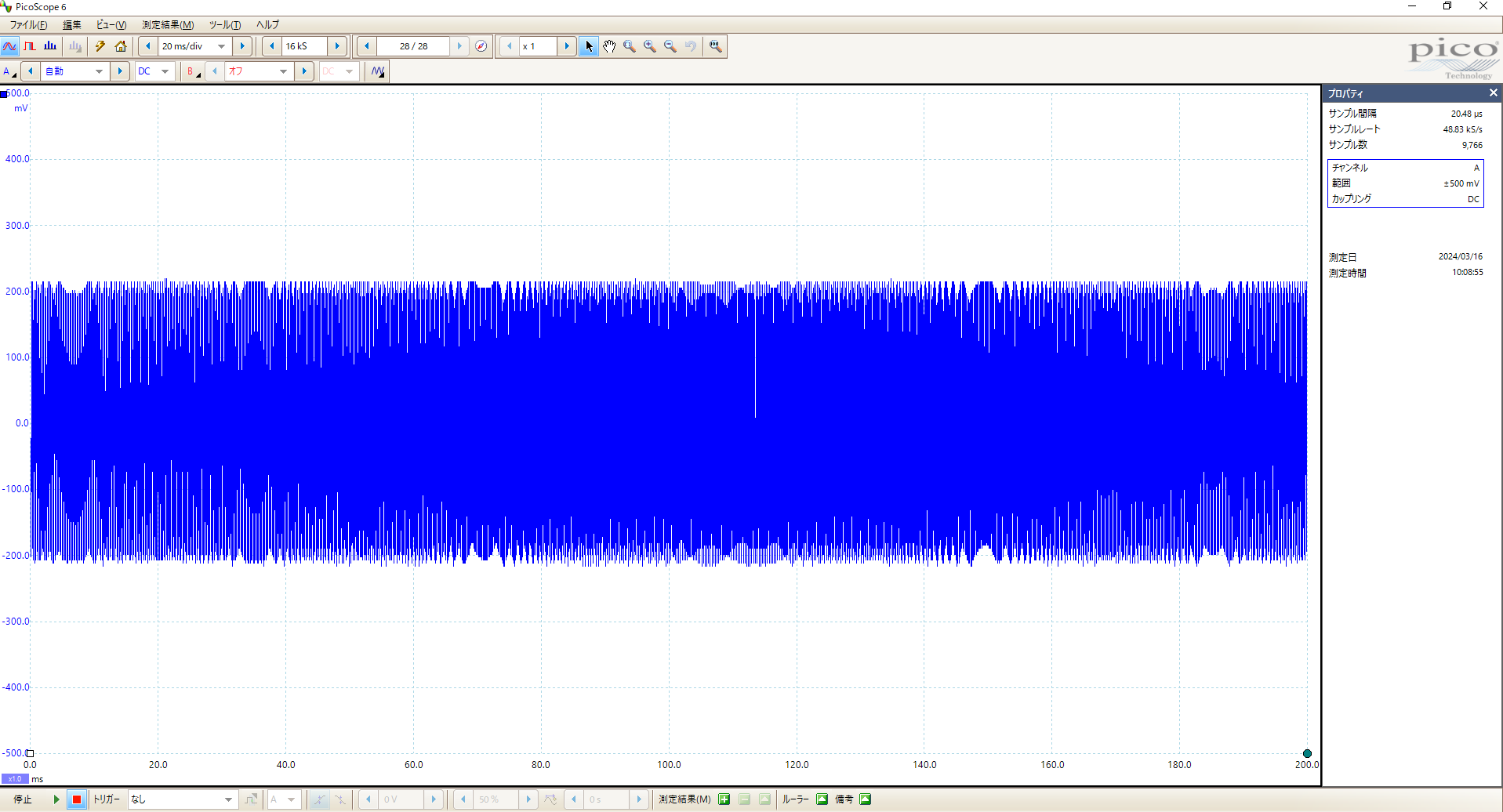
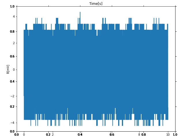
PicoScopeで計測したデータがこちら
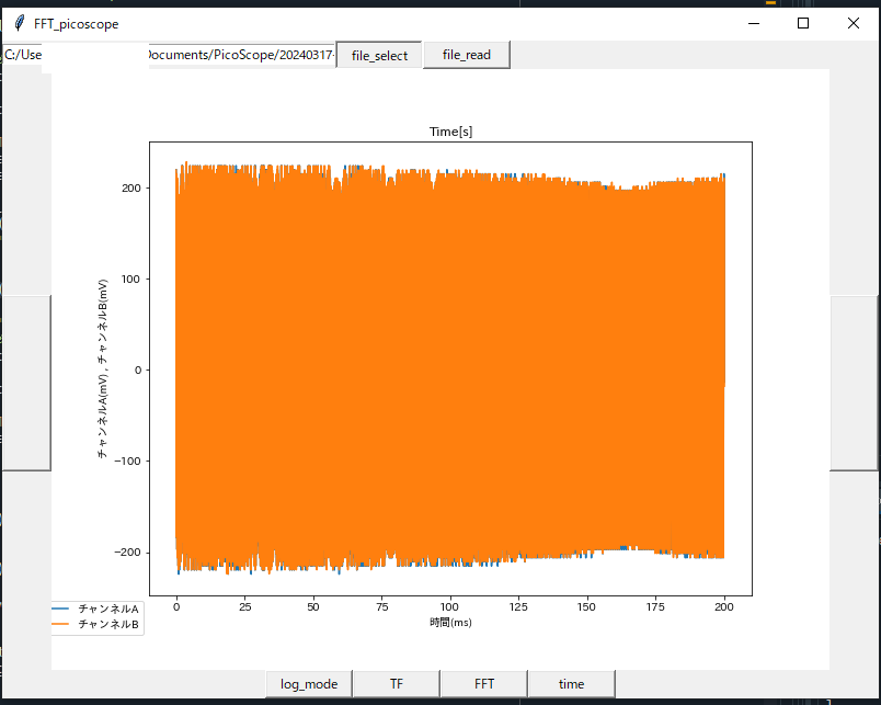
完成したソフト:時系列表示
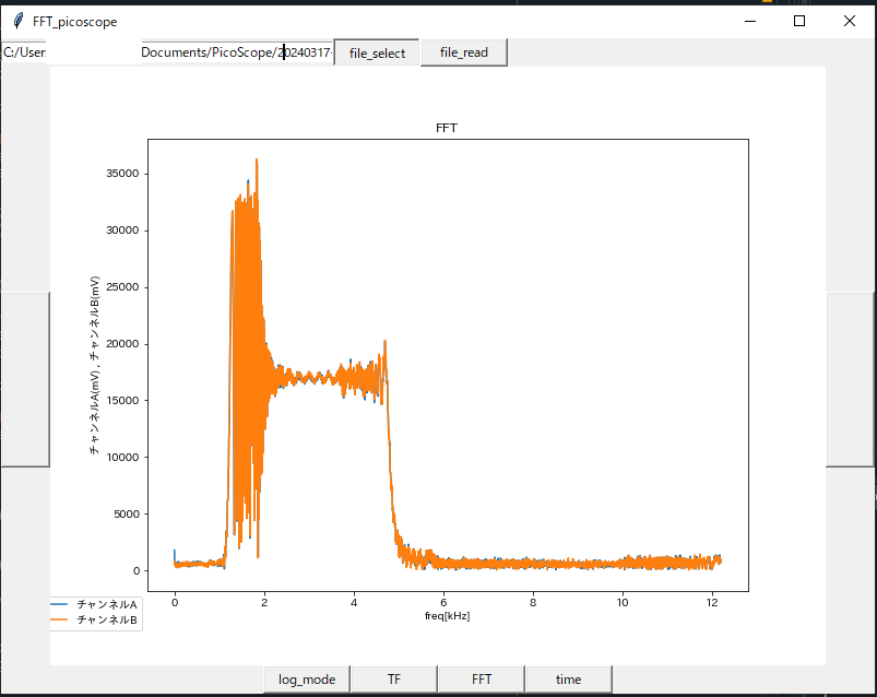
FFT結果表示
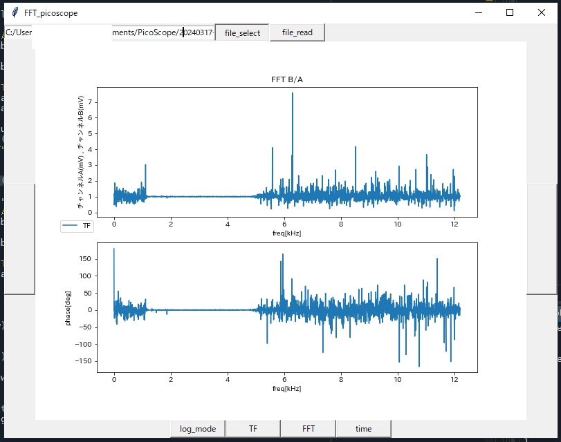
伝達関数計算結果表示
とりあえず欲しいデータ表示はできるようになりました。ここまで工数12h、久々にPython書いたけど思い通りにいかないところが多くて大変だった。
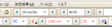
picoscopeの設定
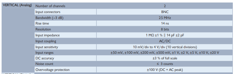
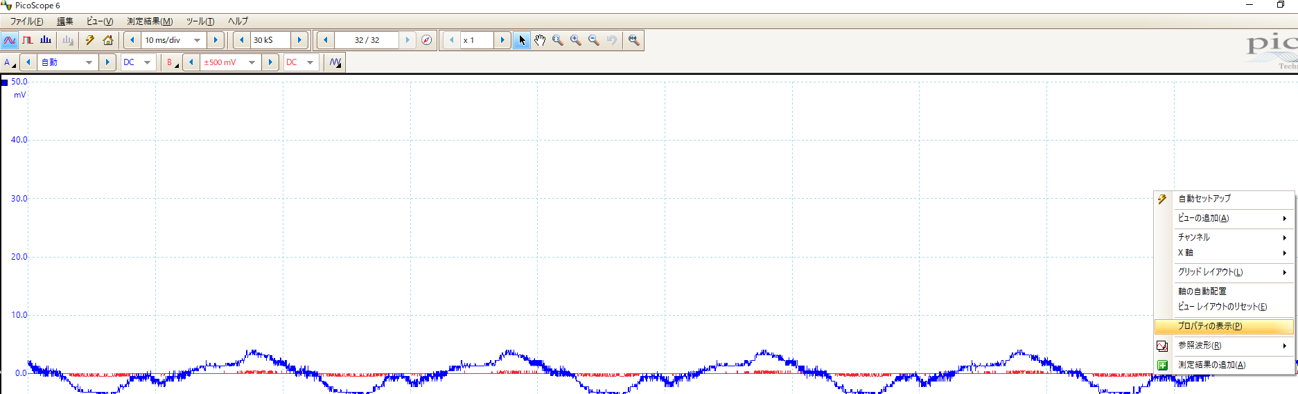
画面右クリックで設定確認可能
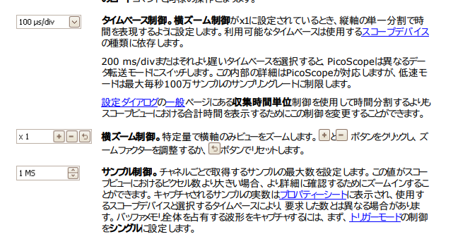
kSの項目はおそらくサンプル[S]の数ただし、実際にはもっと大きい可能性があるみたいだ。
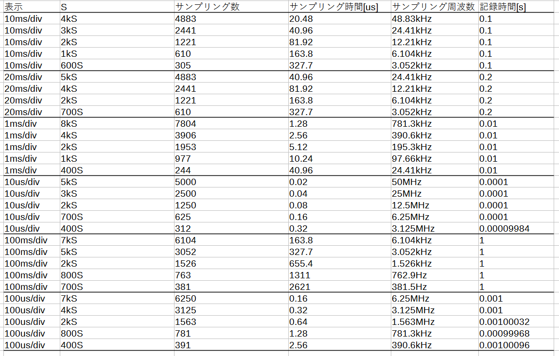
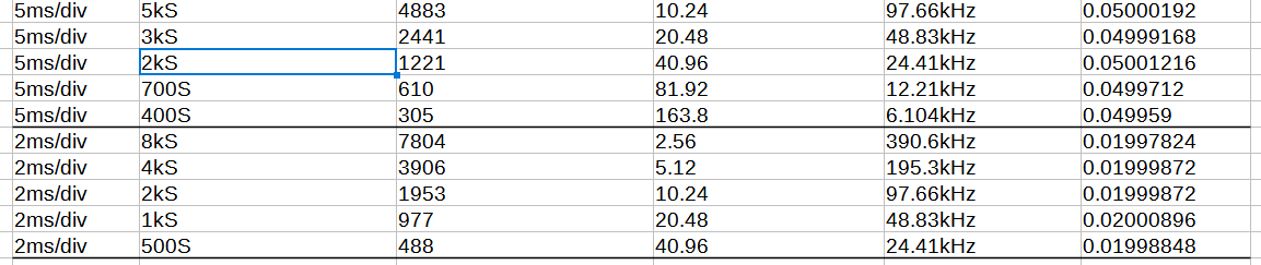
表示用の選択肢[mV/div]ではサンプリング周波数は固定されないみたいだ。
ただし、記録時間は[mV/div]により固定される。高周波・長時間の計測はできない可能性が高い。
一度の計測で最大32フレーム取得できるため、記録時間は最大32倍。ただ、各フレームの接続は連続ではない可能性が高いと思っている。
完成したプログラム
# -*- coding: utf-8 -*
mport sys
import tkinter as tk
import tkinter.filedialog

import pandas as pd
import os
import glob

import matplotlib as mpl
import matplotlib.pyplot as plt
from matplotlib.backends.backend_tkagg import FigureCanvasTkAgg
import japanize_matplotlib

import keyboard
from scipy.fftpack import fft
import numpy as np


root = tk.Tk()

root.title(u"FFT_picoscope")
root.geometry("800x600")

df_list =[]
graph_now = 0
graph_mode = "time"
log_mode = True
TF_mode = True
unit = []

def file_read():

    # ファイル選択ダイアログの表示
    file_path = tkinter.filedialog.askdirectory(initialdir = u"C:/Users/Documents/PicoScope/")

    global df_list
    df_list = []
    global graph_now
    graph_now = 0

    return file_path

def file_select1(event):
    # ファイル選択ダイアログの表示
    data = file_read()
    txtBox_read_file.delete(0,tk.END)
    txtBox_read_file.insert(tk.END,data)

def file_data(event):
    #ファイルのエクセルデータを読み出す
    files =  glob.glob(txtBox_read_file.get()+"/*csv")
    print(files)

    for i in files:
        #dir_txt = txtBox_read_file.get() +"/"+ i
        print(i)
        df = pd.read_csv(i)

        #df.set_index("index",inplace=True)
        global unit
        unit = df.iloc[0,:].to_numpy()
        unit = df.columns.to_numpy() + unit #チャンネルA + mVみたいな演算してるわよ
        df = df.drop(index=0,axis = 0)

        try:
            for i in df.columns:
                df[i] = df[i].str.replace('∞','5')
            df = df.astype(float)
            df_list.append(df)

        except ValueError:
            print("error")


    #df.columns
    #df.dtypes
    global graph_mode
    graph_mode = "time"

    global fig
    global canvas

    if 'ax1' in globals():
        global ax1
        ax1.clear()
        ax1.cla()
        fig.delaxes(ax1)
    if 'ax2' in globals():
        global ax2
        ax2.clear()
        ax2.cla()
        fig.delaxes(ax2)
    canvas.draw()

    # ax1
    ax1 = fig.add_subplot(111)
    ax1.set_title('Time')
    ax1.set_xlabel(unit[0])
    ax1.set_ylabel(unit[1])

    ax1.plot(df.iloc[:,0], df.iloc[:,1])
    if len(df.columns) == 3:
        ax1.set_ylabel(unit[1] + " , " + unit[2] )
        ax1.plot(df.iloc[:,0], df.iloc[:,2])
        ax1.legend([df.columns[1],df.columns[2]],bbox_to_anchor=(0, 0))
    else:
        ax1.legend([df.columns[1]],bbox_to_anchor=(1, 1))

    canvas.draw()

def graph_next(event):
    global graph_now
    global df_list


    if graph_now >= len(df_list)-1:
        return

    else:
        graph_now = graph_now + 1

        global graph_mode
        if graph_mode == "time":
            draw_graph_time()
        elif graph_mode == "fft":
            draw_graph_fft()
        else:
            draw_graph_tf()

def graph_before(event):
    global graph_now
    global df_list


    if graph_now < 1:
        return

    else:
        graph_now = graph_now - 1

        global graph_mode
        if graph_mode == "time":
            draw_graph_time()
        elif graph_mode == "fft":
            draw_graph_fft()
        else:
            draw_graph_tf()

def graph_time(event):
    global graph_mode
    graph_mode = "time"

    draw_graph_time()

def graph_fft(event):
    global graph_mode
    graph_mode = "fft"
    draw_graph_fft()

def log_mode_f(event):
    global log_mode
    log_mode = not(log_mode)

    global graph_mode
    if graph_mode == "fft":
        draw_graph_fft()
    elif graph_mode == "tf":
        draw_graph_tf()

def graph_tf(event):
    global graph_now
    global df_list

    for i in df_list:
        if len(i.columns) != 3:
            print("can not caluculate for 1 axis data")
            return

    global graph_mode
    global TF_mode

    if graph_mode != "tf":
        graph_mode = "tf"
        TF_mode = True
    else:
        TF_mode = not(TF_mode)

    draw_graph_tf()

def draw_graph_time():
    global graph_now
    global df_list

    df = df_list[graph_now]

    #fig = plt.Figure(figsize = (30,20))
    global fig
    global canvas
    global ax1
    ax1.clear()
    ax1.cla()
    fig.delaxes(ax1)

    if 'ax2' in globals():
        try:
            global ax2
            ax2.clear()
            ax2.cla()
            fig.delaxes(ax2)
        except:
            print("ax2 clear error")
    canvas.draw()

    # ax1
    ax1 = fig.add_subplot(111)
    ax1.set_title('Time[s]')
    ax1.set_xlabel(unit[0])
    ax1.set_ylabel(unit[1])

    ax1.plot(df.iloc[:,0], df.iloc[:,1])
    if len(df.columns) == 3:
        ax1.set_ylabel(unit[1] + " , " + unit[2] )
        ax1.plot(df.iloc[:,0], df.iloc[:,2])
        ax1.legend([df.columns[1],df.columns[2]],bbox_to_anchor=(0, 0))
    else:
        ax1.legend([df.columns[1]],bbox_to_anchor=(0, 0))

    canvas.draw()

    print("fin")
    print(graph_now)

def draw_graph_tf():
    global graph_now
    global df_list

    chan_A = df_list[graph_now].iloc[:,1].to_numpy()
    chan_B = df_list[graph_now].iloc[:,2].to_numpy()
    time = df_list[graph_now].iloc[:,0].to_numpy()

    N = len(chan_A)
    A = fft(chan_A,N)
    B = fft(chan_B,N)

    if TF_mode == True:
        TF = A / B
    else:
        TF = B / A

    dt = (time[len(time)-1] - time[0])/len(time)
    df = 1.0/dt /N

    sampleIndex = np.arange(start=0, stop=N)
    f = sampleIndex * df

    global fig
    global canvas
    global ax1
    ax1.clear()
    ax1.cla()
    fig.delaxes(ax1)

    if 'ax2' in globals():
        try:
            global ax2
            ax2.clear()
            ax2.cla()
            fig.delaxes(ax2)
        except:
            print("ax2 clear error")

    canvas.draw()

    # ゲイングラフ ax1
    ax1 = fig.add_subplot(211)
    ax2 = fig.add_subplot(212)

    if TF_mode == True:
        ax1.set_title('FFT' +' A/B')
    else:
        ax1.set_title('FFT' +' B/A')

    if unit[0] == '時間(ms)':
        ax1.set_xlabel('freq[kHz]')
    else:
        ax1.set_xlabel('freq[Hz]')

    if log_mode == True:
        ax1.set_xscale("log")
        ax1.set_yscale("log")

    ax1.set_ylabel(unit[1] + " , " + unit[2] )
    ax1.plot(f[:int(N/2)], np.abs(TF[:int(N/2)]))
    ax1.legend(["TF"],bbox_to_anchor=(0, 0))

    # 位相グラフ ax2
    ax2.plot(f[:int(N/2)],  np.angle(TF[:int(N/2)])*180/np.pi)

    ax2.set_ylabel("phase[deg]")
    if unit[0] == '時間(ms)':
        ax2.set_xlabel('freq[kHz]')
    else:
        ax2.set_xlabel('freq[Hz]')

    if log_mode == True:
        ax2.set_xscale("log")

    canvas.draw()

    print("fin")
    print(graph_now)


def draw_graph_fft():
    #fft処理とグラフ表示
    global graph_now
    global df_list

    chan_A = df_list[graph_now].iloc[:,1].to_numpy()
    time = df_list[graph_now].iloc[:,0].to_numpy()

    N = len(chan_A)
    X = fft(chan_A,N)
    if len(df_list[graph_now].columns) == 3:
        chan_B = df_list[graph_now].iloc[:,2].to_numpy()
        Y = fft(chan_B,N)

    dt = (time[len(time)-1] - time[0])/len(time)
    df = 1.0/dt /N

    sampleIndex = np.arange(start=0, stop=N)
    f = sampleIndex * df

    #列が2つのときは

    #fig = plt.Figure(figsize = (30,20))
    global fig
    global canvas
    global ax1
    ax1.clear()
    ax1.cla()
    fig.delaxes(ax1)
    if 'ax2' in globals():
        try:
            global ax2
            ax2.clear()
            ax2.cla()
            fig.delaxes(ax2)
        except:
            print("ax2 clear error")
    canvas.draw()

    # ax1
    ax1 = fig.add_subplot(111)
    ax1.set_title('FFT')
    if unit[0] == '時間(ms)':
        ax1.set_xlabel('freq[kHz]')
    else:
        ax1.set_xlabel('freq[Hz]')

    ax1.set_ylabel(unit[1])

    if log_mode == True:
        ax1.set_xscale("log")
        ax1.set_yscale("log")

    df = df_list[graph_now]

    ax1.plot(f[:int(N/2)], np.abs(X[:int(N/2)]))
    if len(df_list[graph_now].columns) == 3:
        ax1.set_ylabel(unit[1] + " , " + unit[2] )
        ax1.plot(f[:int(N/2)], np.abs(Y[:int(N/2)]))
        ax1.legend([df.columns[1],df.columns[2]],bbox_to_anchor=(0, 0))
    else:
        ax1.legend([df.columns[1]],bbox_to_anchor=(0, 0))

    canvas.draw()

    print("fin")
    print(graph_now)


frame1 = tk.Frame(root)
frame1.pack(anchor=tk.W)


#ファイル場所
txtBox_read_file = tk.Entry(frame1)
txtBox_read_file.configure(state = 'normal',width = 50)
#txtBox_read_file.grid(row = 0,column = 1,padx = 5,pady = 5)
txtBox_read_file.pack(side = 'left')

#ファイル選択ボタン
button1 = tk.Button(frame1,text = 'file_select',width = 10)
#button1.grid(row = 0,column = 2,padx = 5,pady = 5)
button1.bind('<Button-1>',file_select1)
button1.pack(side = 'left')

#データ読み込みボタン
button2 = tk.Button(text = 'file_read',width = 10)
#button2.grid(row = 1,column = 1,padx = 5,pady = 5)
button2.bind('<Button-1>',file_data)
button2.pack(side = 'top',anchor=tkinter.N,after=button1)


#次のグラフボタン
button_n = tk.Button(height = 10,width = 5)
button_n.bind('<Button-1>',graph_next)
button_n.pack(side = 'right')

#前のグラフボタン
button_b = tk.Button(height = 10,width = 5)
button_b.bind('<Button-1>',graph_before)
button_b.pack(side = 'left')

frame2 = tk.Frame(root)
frame2.pack(side = 'bottom',anchor = tk.S)

#log_modeボタン
button_log = tk.Button(frame2,width = 10,text = 'log_mode')
button_log.bind('<Button-1>',log_mode_f)
button_log.pack(side = 'left')

#FFTボタン
button_fft = tk.Button(frame2,width = 10,text = 'FFT')
button_fft.bind('<Button-1>',graph_fft)
button_fft.pack(side = 'left')

#TFボタン
button_tf = tk.Button(frame2,width = 10,text = 'TF')
button_tf.bind('<Button-1>',graph_tf)
button_tf.pack(side = 'left',before = button_fft)

#timeボタン
button_time = tk.Button(frame2,width = 10,text = 'time')
button_time.bind('<Button-1>',graph_time)
button_time.pack(side ='left')


#canvas
fig = plt.Figure(figsize = (30,20))
canvas = FigureCanvasTkAgg(fig, master=root)
canvas.get_tk_widget().pack(side = 'top')


root.mainloop()
スイープ波(SWEPT SIN)のFFTについて
(スイープとSWEPT SINとチャープ信号に違いがあるのか?)
\begin{eqnarray}
f = ASin(wt)\\
w = w_0 + \alpha t
\end{eqnarray}
をDFTしたい。
数式的答えは調べても見つからなかった・・・
\begin{eqnarray}
F[k] = \sum_{n=0}^{N-1} f[n] e^{-j \frac{2\pi}{N} kn}
\end{eqnarray}
基本的なDFT結果を見てみよう。
sin(wt)のDFT
$\sin( \omega_0 t)$のフーリエ変換はデルタ関数$\delta(\omega - \omega_0) + \delta(\omega + \omega_0)$になる。
離散信号$\sin( \omega_0 n)$のDFTは$F[k] = 1(k = \omega_0),0(else)$になる。
数式的に求める。
\begin{eqnarray}
F[k] &=& \sum_{n=0}^{N-1} \sin( \omega n) e^{-j \frac{2\pi}{N} kn}\\
&=& \sum_{n=0}^{N-1} \frac{e^{ j \omega n} - e^{ - j \omega n}}{2j} e^{-j \frac{2\pi}{N} kn}\\
&=& \sum_{n=0}^{N-1} \frac{e^{ j \omega n-j \frac{2\pi}{N} kn} - e^{ - j \omega n -j \frac{2\pi}{N} kn}}{2j} \\
&=& \sum_{n=0}^{N-1} \frac{e^{ j (\omega - \frac{2\pi}{N} k)n} - e^{ - j (\omega  + \frac{2\pi}{N} k)n}}{2j} \\
\end{eqnarray}
指数部が0でないと総和は0になると考えられる(理由は後述)。
よって、
\begin{eqnarray}
F[k] =

\left\{
\begin{array}{ll}
-N/2j & (k= \frac{\omega N}{2 \pi})\\
0 & (else)
\end{array}
\right.
\end{eqnarray}
(理由)
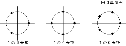
1の4️乗の点の総和は0になる。逆に、3乗、5乗は0にならない。
- 指数部が整数周する
- 1周の点数が偶数である
以上2つの条件が必要。
\begin{eqnarray}
k &=& 0,1,\cdots ,N-1(上の式ではどれかの固定値)\\
n &=& 0,1,\cdots ,N-1\\
\omega &=& g \frac{2\pi}{N}(gは整数とする)\\
&N&が偶数
\end{eqnarray}
こう考えると次のように式変形できる。
\begin{eqnarray}
F[k] &=& \sum_{n=0}^{N-1} \frac{e^{ j (g - k) \frac{2\pi}{N} n} - e^{ - j (g  +  k) \frac{2\pi}{N} n}}{2j} \\
\end{eqnarray}
指数部がまとまることにより「整数周すること」、$N$が偶数であることにより「1周の点数が偶数である」ことが満たされる。
(追記)
\omega = g \frac{2\pi}{N}(gは整数とする)\\
この制約はかなりきつい。信号が計測期間$n = 0,\cdots ,N$でちょうど位相が一致することを意味しているからだ。
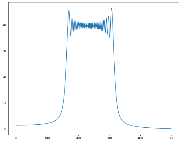
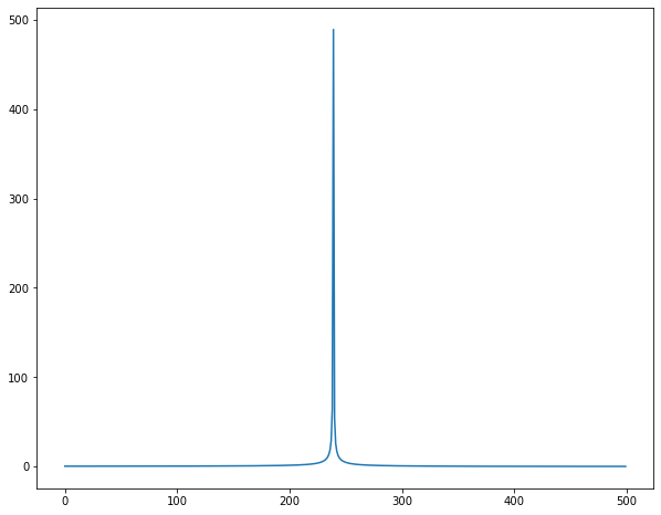
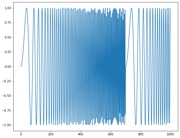
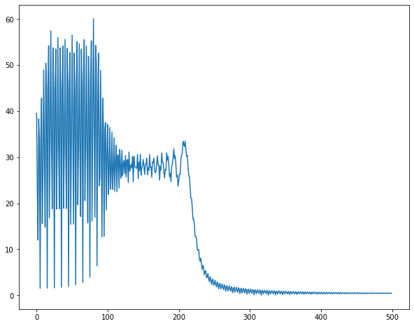
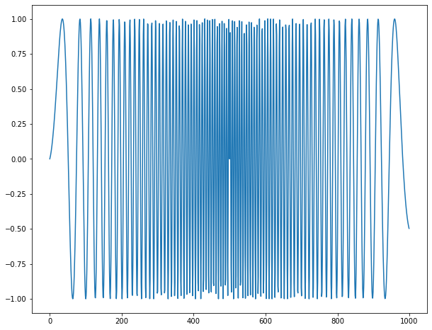
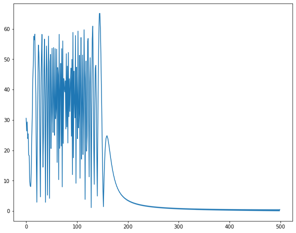
Pythonでスイープ波のDFT結果
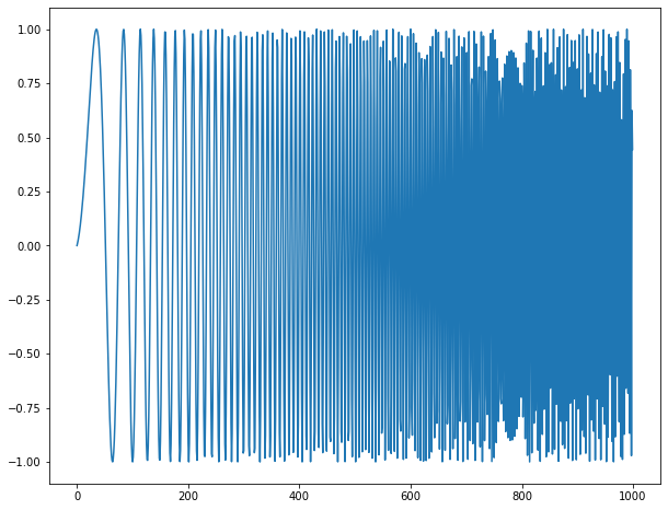
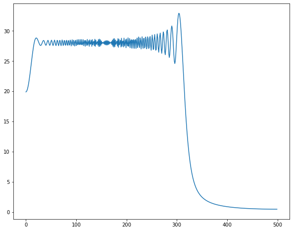
以下のように設定した結果
\begin{eqnarray}
f = A \sin(\omega n)\\
\omega = \omega_0 + \alpha n\\
n = 0,\cdots,999\\
\omega_0 = 0.01\\
\alpha = 0.001\\
\omega = 0.01,\cdots,1.01(正しくは2.01,理由は後述)
\end{eqnarray}
最小正規化角周波数$2\pi / N$は$6.28\times 10^{-3}$
スペクトルグラフの横軸は$n$を表しており、$n \times 2\pi / N$が正規化角周波数である(正規化角周波数は$0,\cdots,2 \pi$で変動)。
import functools
import matplotlib.pyplot as plt
import cmath
import random

import numpy as np

def dft(f):
    n = len(f)
    Y = []
    for x in range(n):
        y = 0j
        for t in range(n):
            a = 2 * cmath.pi * t * x / n
            y += f[t] * cmath.e**(-1j * a)
        Y.append(y)
    return Y

n = np.arange(1000)
omega_0 = 0.01
alpha = 0.001

y = np.sin((omega_0 + alpha*n)* n)

fig = plt.figure(figsize = (10,8))
ax1 = fig.add_subplot(111)
ax1.plot(n, y)
#plt.show()


fy = np.array(dft(y))
fig2 = plt.figure(figsize = (10,8))
ax2 = fig2.add_subplot(111)
ax2.plot(np.abs(fy)[:int(len(fy)/2)])
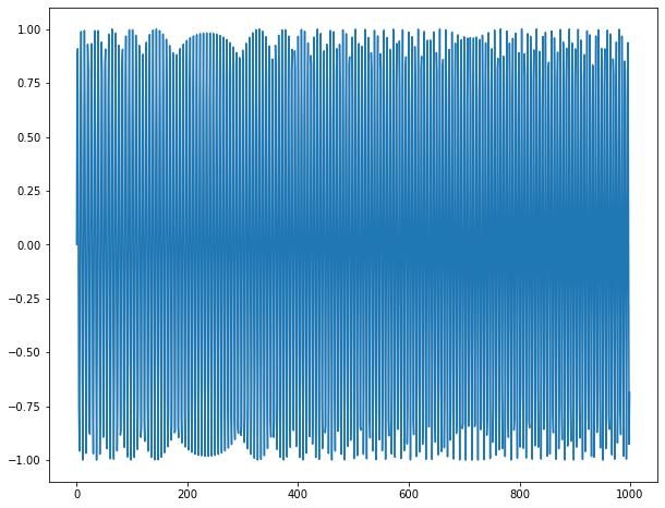
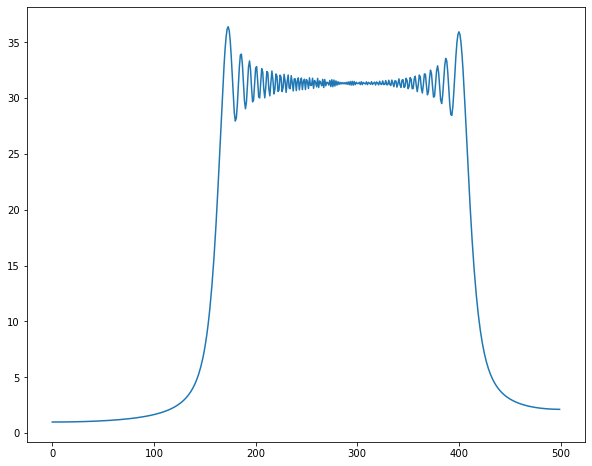
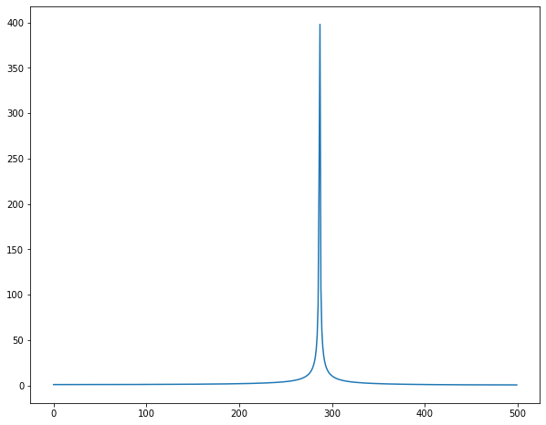
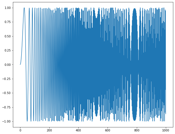
場合2
n = np.arange(1000)
omega_0 = 1.0
alpha = 0.0001

y = np.sin((omega_0 + alpha*n)* n)
\begin{eqnarray}
f = A \sin(\omega n)\\
\omega = \omega_0 + \alpha n\\
n = 0,\cdots,999\\
\omega_0 = 1.0\\
\alpha = 0.0001\\
\omega = 1.0,\cdots,1.1(正しくは1.2)\\
\end{eqnarray}
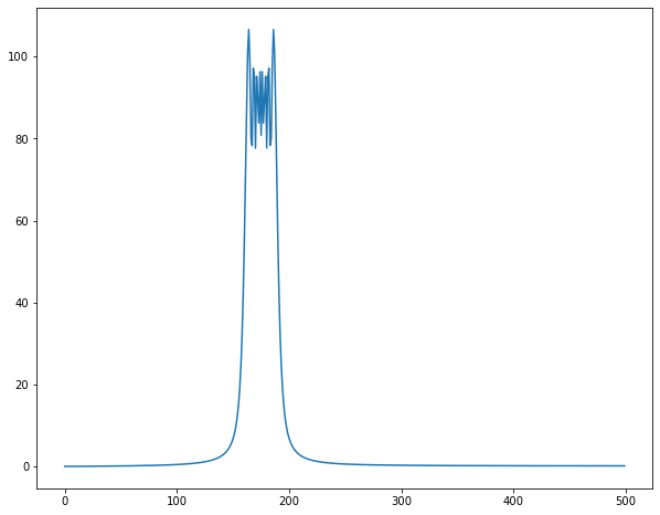
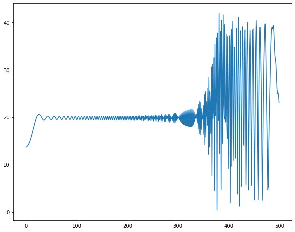
正規化角周波数のなぞ

\begin{eqnarray}
\omega = 1.0,\cdots,1.1\\
\end{eqnarray}
\begin{eqnarray}
\omega = 1.0,\cdots,1.2\\
\end{eqnarray}
\begin{eqnarray}
\omega = 1.0,\cdots,1.5\\
\end{eqnarray}
\begin{eqnarray}
\omega =1.5\\
\end{eqnarray}
なんか位置があわないなぁ・・・
よく見たら、$\omega = 1.0,\cdots,1.5$のグラフの中央が$\omega = 1.5$の値じゃないか!?
\begin{eqnarray}
f = A \sin(\omega n)\\
\omega = \omega_0 + \alpha n\\
\end{eqnarray}
これで生成するチャープ信号の周波数成分は
\omega = \omega_0 , \cdots , \omega_0 + \alpha N\\
と考えていたが、
\omega = \omega_0 , \cdots , \omega_0 + 2\alpha N\\
になるのか?
$\sin( \omega t^2)$を時刻$t_0$に微小区間$dt$で捉えた時($t_0 >> dt$)の信号は $sin(\omega t_0^2 + 2 \omega t_0 dt) = Asin(2\omega t_0 dt)$となる。つまり、周波数は$2\omega t_0$ということになる?
あってる?
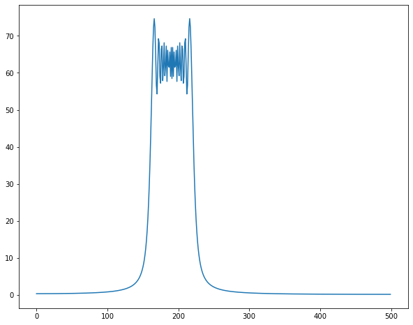
\begin{eqnarray}
\omega = 1.0,\cdots,1.8\\
\end{eqnarray}
は間違いで、
\begin{eqnarray}
\omega = 1.0,\cdots,2.6\\
\end{eqnarray}
が正しいはず
\begin{eqnarray}
\omega =1.8\\
\end{eqnarray}
チャープ信号の周期と計測区間に食い違いがある場合
チャープ信号の途中で$w_0$に戻る場合を考えてみます。
低周波領域がギザギザするようになりました。数学的考えると原因は明らかです。
- チャープ信号の低周波領域がFFT区間に複数混ざっています。時間遅れ信号は周波数帯域では$e^{-jwT}$かかることになります。振幅に変化は与えず、位相のみがずれます。
- $f = f_1 + f_2$のフーリエ変換は$F(w) = F_1(w) + F_2(w) $です。「信号の足し合わせ」=「フーリエ変換の足し合わせ」です。
以上2つから低周波領域において、元の周波数領域成分$F(jw)$と時間遅れ要素$e^{-jwT}$がかかったデータ$F(jw)e^{-jwT}$2つの和になり、$|F(jw)(1+e^{-jwT})| =F(w) \times abs( 1+e^{-jwT})$となります。
$1+abs( 1+e^{-jwT})$は周波数で振動するため、低周波領域ではギザギザが現れたのでしょう・・・
振動の振幅は0~2であるため、実験結果も倍率は0~2になっています!
チャープ信号がサンプリング周波数/2を超える時
n = np.arange(1000)
omega_0 = 0.001
alpha = 0.002
k = np.arange(1000)
y = np.sin((omega_0 + alpha*k)* k)
サンプリングの定理から、サンプリング周波数/2を超える信号は折り返し、高周波数領域の信号が時間遅れで追加されるのと同じ状況になります。
FFT結果も高周波領域に対し$1+abs( 1+e^{-jwT})$がかかっている結果になっていますねwww
特殊チャープ信号
周波数が上がって、半分から下がりもとに戻る
時間遅れ要素がかかるため結局ぎざぎざになる・・・
サンプリング周波数と必要帯域
サンプリングの定理によれば、アナログの信号側の2倍のサンプリング周波数があれば良いはずです。しかし、リンクのサイトによると帯域の30%を超えると振幅が減少するそうです。
計測可能な立ち上がり時間より早く立ち上がると正しく観測できなくなるためだそうです。
プローブの校正
校正をちゃんとしないと正しい周波数特性が得られません。
*10でプローブを運用したほうが精度がいいのかな・・・
tkinterとmatplotlibでグラフを更新したいときのつまずき
グラフを表示しようとしたときに、前書いたグラフが重なってしまったときの対処法です。
解決策
        global fig
        global canvas
        global ax1
        ax1.clear()
        ax1.cla()
        fig.delaxes(ax1)
        canvas.draw()
削除して一度、canvasを再drawしてリセットする。
その後、再度plotしてdrawする。