【R入門】R言語の基本:2変数の記述統計

統計とR言語の勉強をしています。
「Rによるやさしい統計学」の写経で勉強。

実行環境

• Windows10 Pro 64bit
• R：3.4.3
• RStudio：1.1.383

RStudioのConsoleを使って実行しています

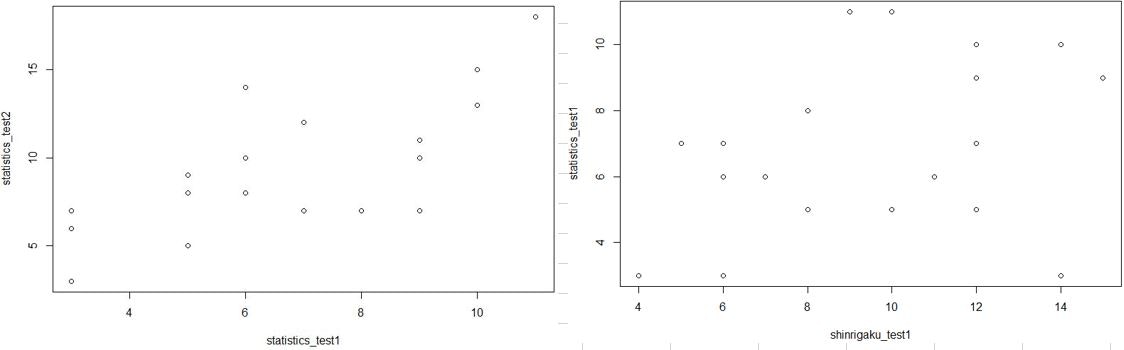
散布図

2変数の散布図出力。

> shinrigaku_test1 <- c(11, 14, 7, 12, 10, 6, 8,15, 4, 14, 9, 6, 10, 12, 5, 12, 8, 6, 12, 15)
> statistics_test1 <- c(6, 10, 6, 10, 5, 3, 5, 9, 3, 3, 11, 6, 11, 9, 7, 5, 8, 7, 7, 9)
> statistics_test2 <- c(10, 13, 8, 15, 8, 6, 9, 10, 7, 3, 18, 14, 18, 11, 12, 5, 7,12, 7, 7)
> plot(statistics_test1,statistics_test2)
> plot(shinrigaku_test1,statistics_test1)

共分散

「偏差の積の平均」である共分散の出力。上のコードの続きです。
地味に計算します。

> kyoubunsan1_2 <- sum((statistics_test1-mean(statistics_test1))*(statistics_test2-mean(statistics_test2)))/length(statistics_test1)
> kyoubunsan1_2
[1] 7.55

共分散はcov関数で算出できるのですが、不偏共分散なので上の結果の7.55と異なります。

> cov(statistics_test1,statistics_test2)
[1] 7.947368

相関係数

相関係数は、共分散を標準偏差の積で割ったものです。cor関数で算出できます。

> #地味計算
> cov(statistics_test1,statistics_test2)/(sd(statistics_test1)*sd(statistics_test2))
[1] 0.749659
> #using cor function
> cor(statistics_test1,statistics_test2)
[1] 0.749659

クロス集計表

table関数を使ってクロス集計表を出力。

> math <- c("嫌い","嫌い","好き","好き","嫌い","嫌い","嫌い","嫌い","嫌い","好き","好き","嫌い","好き","嫌い","嫌い","好き","嫌い","嫌い","嫌い","嫌い")
> table(math)
math
嫌い 好き 
  14    6 
> stat <- c("好き","好き","好き","好き","嫌い","嫌い","嫌い","嫌い","嫌い","嫌い","好き","好き","好き","嫌い","好き","嫌い","嫌い","嫌い","嫌い","嫌い")
> table(stat)
stat
嫌い 好き 
  12    8 
> table(math,stat)
      stat
math   嫌い 好き
  嫌い   10    4
  好き    2    4

ファイ係数

1と0の2つの値からなる変数に対して計算される相関係数をファイ係数と呼びます。
ifelse関数を使ってテキストを1/0に変換して相関係数を計算することでファイ係数を算出します。

> math10 <- ifelse(math=="好き",1,0)
> math10
 [1] 0 0 1 1 0 0 0 0 0 1 1 0 1 0 0 1 0 0 0 0
> stat10 <- ifelse(stat=="好き",1,0)
> stat10
 [1] 1 1 1 1 0 0 0 0 0 0 1 1 1 0 1 0 0 0 0 0
> cor(math10, stat10)
[1] 0.3563483