- 製造業出身のデータサイエンティストがお送りする記事
- 今回はクラスタリング手法の中で、K-means法を実装しました。
クラスタリングとは
クラスタリングとは、ある集合を何らかの規則によって分類することです。機械学習においてクラスタリングは、「教師なし学習」に分類されます。
クラスタリングの計算方法はいくつかありますが、サンプル同士の類似性に基づいてグルーピングしています。クラスタリングの計算方法を大きく分類すると、「階層クラスタリング」と「非階層クラスタリング」の2つに分けられます。
今回実装するK-means法は「非階層クラスタリング」に分類されます。
K-means法とは
クラスターの平均を用いて、あらかじめ決められたクラスター数に分類手法です。K-means法のアルゴリズム概要は下記にようになっております。
- クラスタの中心の初期値をk個決める
- 全てのサンプルとk個のクラスタとの中心距離を求め、最も近いクラスタに分類する
- 形成されたk個のクラスタの中心を求める
- 中心が変化しなくなるまで2と3の工程を繰り返す

K-means法の実装
pythonのコードは下記の通りです。
# 必要なライブラリーのインストール
import numpy as np
import pandas as pd

# 可視化
import matplotlib as mpl
import matplotlib.pyplot as plt
import seaborn as sns
from IPython.display import display
%matplotlib inline
sns.set_style('whitegrid')

# 正規化のためのクラス
from sklearn.preprocessing import StandardScaler

# k-means法に必要なものをインポート
from sklearn.cluster import KMeans
最初に必要なライブラリーをimportします。
今回はirisのデータを使って実装してみようと思います。
# irisデータ
from sklearn.datasets import load_iris

# データ読み込み
iris = load_iris()
iris.keys()

# データフレームに格納
df_iris = pd.DataFrame(iris.data, columns=iris.feature_names)
df_iris['target'] = iris.target # アヤメの種類(正解ラベル)
df_iris.head()

# 2変数の散布図(正解ラベルで色分け)
plt.scatter(df_iris['petal length (cm)'], df_iris['petal width (cm)'], c=df_iris.target, cmap=mpl.cm.jet)
plt.xlabel('petal_length')
plt.ylabel('petal_width')
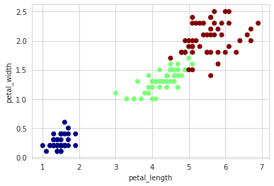
「petal_length」と「petal_width」の2変数で可視化してみました。
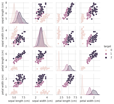
次に散布図行列で可視化してみたいと思います。
# 散布図行列(正解ラベルで色分け)
sns.pairplot(df_iris, hue='target', height=1.5)
次にエルボー法を用いて、クラスタ数を決めていきたいと思います。irisのデータだと3個に分ければ良いことは明確ですが、実際クラスタリングを使用する時は教師なし学習のため、クラスタ数を自分で決めなければいけません。そこで、クラスタ数を決めるための手法の一つとしてエルボー法があります。
# Elbow Method
wcss = []

for i in range(1, 10):
    kmeans = KMeans(n_clusters = i, init = 'k-means++', max_iter = 300, n_init = 30, random_state = 0)
    kmeans.fit(df_iris.iloc[:, 2:4])
    wcss.append(kmeans.inertia_)


plt.plot(range(1, 10), wcss)
plt.title('The elbow method')
plt.xlabel('Number of clusters')
plt.ylabel('WCSS')
plt.show()

エルボー法の結果を見ても、クラスタ数は3以上増やしても意味がないことがわかるかと思います。
ここからモデリングをしていきたいと思います。
# モデリング
clf = KMeans(n_clusters=3, random_state=1)
clf.fit(df_iris.iloc[:, 2:4])

# 学習データのクラスタ番号
clf.labels_

# 未知データに対してクラスタ番号を付与
# 今回は学習データに対して予測しているので、`clf.labels_` と同じ結果
y_pred = clf.predict(df_iris.iloc[:, 2:4])
y_pred

# 実際の種類とクラスタリングの結果を比較
fig, (ax1, ax2) = plt.subplots(figsize=(16, 4), ncols=2)

# 実際の種類の分布
ax1.scatter(df_iris['petal length (cm)'], df_iris['petal width (cm)'], c=df_iris.target, cmap=mpl.cm.jet)
ax1.set_xlabel('petal_length')
ax1.set_ylabel('petal_width')
ax1.set_title('Actual')
# クラスター分析で分類されたクラスタの分布
ax2.scatter(df_iris['petal length (cm)'], df_iris['petal width (cm)'], c=y_pred, cmap=mpl.cm.jet)
ax2.set_xlabel('petal_length')
ax2.set_ylabel('petal_width')
ax2.set_title('Predict')

さいごに
最後まで読んで頂き、ありがとうございました。
今回は、K-means法を実装しました。
訂正要望がありましたら、ご連絡頂けますと幸いです。