PyTorch Geometricを用いたPointNet++の実装例の確認

DeepLearningを用いて点群(point clouds)データを取り扱うにあたってはPointNetの研究が有名です。当記事ではPointNetやPointNetにグラフ畳み込みを導入したPointNet++の理解にあたって、PyTorch Geometric(PyG)を用いた実装について確認します。

前提・基本トピックの確認

PyTorch Geometricのインストール

PyTorch Geometricドキュメント

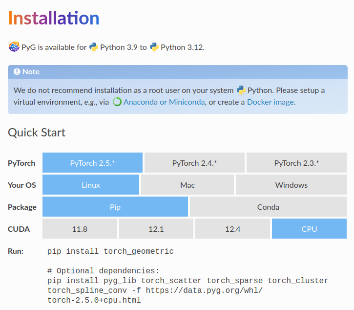
PyTorch Geometricのインストールにあたっては上記に基づいて行えば良いです。OSやCUDAのバージョンなどによってコマンドが変わるので、注意して確認した上でインストールを行うと良いと思います。

GeometricShapesデータセットの確認

当記事ではPointNet++の学習にあたってGeometricShapesデータセットを用いるので以下GeometricShapesデータセットについて簡単に確認します。

from torch_geometric.datasets import GeometricShapes
import matplotlib.pyplot as plt

dataset = GeometricShapes(root='data/GeometricShapes')
data = dataset[0]

print(len(dataset))
print(data)
print(data.pos.shape)

・実行結果

40
Data(pos=[32, 3], face=[3, 30], y=[1])
torch.Size([32, 3])

上記のdatasetは40種類の図形の点群データを持ち、dataのposは各点の3Dの位置、faceは各点からメッシュを構成する際の3点のインデックスをそれぞれ保持します。40種類の図形から10種類だけ下記に列記します。

・2d_circle
・2d_ellipse
・2d_moon
・2d_pacman
・2d_plane
・2d_semicircle
・2d_trapezoid
・2d_triangle
・3d_L_cylinder
・3d_U_cylinder

上記を可視化するにあたっては下記などを実行すると良いです。

import matplotlib.pyplot as plt
from torch_geometric.datasets import GeometricShapes

dataset = GeometricShapes(root='data/GeometricShapes')

for i in range(len(dataset)):
    data = dataset[i]
    fig = plt.figure()
    ax = fig.add_subplot(projection='3d')
    ax.scatter(data.pos.numpy()[:,0], data.pos.numpy()[:,1], data.pos.numpy()[:,2])
    plt.savefig("png/sample{}.png".format(i+1))

・実行結果①(2d_circle: png/sample1.png)

・実行結果②(2d_moon: png/sample3.png)

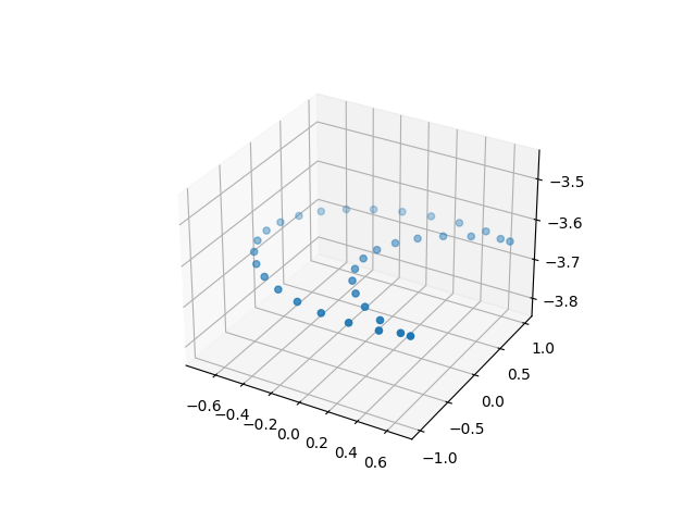
・実行結果③(2d_plane: png/sample5.png)

・実行結果④(2d_triangle: png/sample8.png)

・実行結果⑤(3d_U_cylnder: png/sample10.png)

PyTorch Geometricを用いたPointNet++の実装の確認

PointNetLayerクラスは上記と同様にMessagePassingに基づいて下記のように実装されます。

from torch import Tensor
from torch.nn import Sequential, Linear, ReLU
from torch_geometric.nn import MessagePassing

class PointNetLayer(MessagePassing):
    def __init__(self, in_channels: int, out_channels: int):
        # Message passing with "max" aggregation.
        super().__init__(aggr='max')

        # Initialization of the MLP:
        # Here, the number of input features correspond to the hidden
        # node dimensionality plus point dimensionality (=3).
        self.mlp = Sequential(
            Linear(in_channels + 3, out_channels),
            ReLU(),
            Linear(out_channels, out_channels),
        )

    def forward(self,
        h: Tensor,
        pos: Tensor,
        edge_index: Tensor,
    ) -> Tensor:
        # Start propagating messages.
        return self.propagate(edge_index, h=h, pos=pos)

    def message(self,
        h_j: Tensor,
        pos_j: Tensor,
        pos_i: Tensor,
    ) -> Tensor:
        # h_j: The features of neighbors as shape [num_edges, in_channels]
        # pos_j: The position of neighbors as shape [num_edges, 3]
        # pos_i: The central node position as shape [num_edges, 3]

        edge_feat = torch.cat([h_j, pos_j - pos_i], dim=-1)
        return self.mlp(edge_feat)

上記が一般的なグラフ畳み込みと異なる点はMessage Passingの際のaggregation(super().__init__(aggr='max'))にadd(sumと同義)ではなくmaxを用いているところや、aggregation処理の後のMLP処理の入力にpos_j - pos_iに基づく3つの次元を追加しているところです。__init__関数のself.mlpの計算にあたってLinear(in_channels + 3, out_channels)を計算することで次元の調整を行っていることも合わせて抑えておくと良いです。

PointNetクラスの実装

PointNetクラスは前項のPointNetLayerクラスを元に下記のように実装することができます。

from torch_geometric.nn import global_max_pool

class PointNet(torch.nn.Module):
    def __init__(self):
        super().__init__()

        self.conv1 = PointNetLayer(3, 32)
        self.conv2 = PointNetLayer(32, 32)
        self.classifier = Linear(32, dataset.num_classes)

    def forward(self,
        pos: Tensor,
        edge_index: Tensor,
        batch: Tensor,
    ) -> Tensor:

        # Perform two-layers of message passing:
        h = self.conv1(h=pos, pos=pos, edge_index=edge_index)
        h = h.relu()
        h = self.conv2(h=h, pos=pos, edge_index=edge_index)
        h = h.relu()

        # Global Pooling:
        h = global_max_pool(h, batch)  # [num_examples, hidden_channels]

        # Classifier:
        return self.classifier(h)

上記は基本的には一般的なPyTorch Geometricを用いたグラフニューラルネットワーク(GNN; Graph Neural Network)の実装ではありますが、__init__関数でPointNetLayerが用いられていることが確認できます。また、当記事で解くタスクは「点群(data.x)から点群の分類(data.y)を予測するグラフ分類タスク」であるので、torch_geometric.nn.global_max_poolを用いてプーリングが行われている点も注意しておくと良いです。

学習の実行

学習の実行にあたっては下記のようなコードを動かすと良いです。

from torch_geometric.datasets import GeometricShapes
from torch_geometric.loader import DataLoader
import torch_geometric.transforms as T

dataset = GeometricShapes(root='data/GeometricShapes')
model = PointNet()

train_dataset = GeometricShapes(root='data/GeometricShapes', train=True)
train_dataset.transform = T.Compose([T.SamplePoints(num=256), T.KNNGraph(k=6)])
test_dataset = GeometricShapes(root='data/GeometricShapes', train=False)
test_dataset.transform = T.Compose([T.SamplePoints(num=256), T.KNNGraph(k=6)])

train_loader = DataLoader(train_dataset, batch_size=10, shuffle=True)
test_loader = DataLoader(test_dataset, batch_size=10)

model = PointNet()
optimizer = torch.optim.Adam(model.parameters(), lr=0.01)
criterion = torch.nn.CrossEntropyLoss()


def train():
    model.train()

    total_loss = 0
    for data in train_loader:
        optimizer.zero_grad()
        logits = model(data.pos, data.edge_index, data.batch)
        loss = criterion(logits, data.y)
        loss.backward()
        optimizer.step()
        total_loss += float(loss) * data.num_graphs

    return total_loss / len(train_loader.dataset)

@torch.no_grad()
def test():
    model.eval()

    total_correct = 0
    for data in test_loader:
        logits = model(data.pos, data.edge_index, data.batch)
        pred = logits.argmax(dim=-1)
        total_correct += int((pred == data.y).sum())

    return total_correct / len(test_loader.dataset)


for epoch in range(1, 51):
    loss = train()
    test_acc = test()
    print(f'Epoch: {epoch:02d}, Loss: {loss:.4f}, Test Acc: {test_acc:.4f}')

・実行結果

Epoch: 01, Loss: 3.7448, Test Acc: 0.0250
Epoch: 02, Loss: 3.7014, Test Acc: 0.0250
Epoch: 03, Loss: 3.6850, Test Acc: 0.0500
Epoch: 04, Loss: 3.6487, Test Acc: 0.0750
Epoch: 05, Loss: 3.5888, Test Acc: 0.0250
Epoch: 06, Loss: 3.5487, Test Acc: 0.0250
Epoch: 07, Loss: 3.5116, Test Acc: 0.0500
Epoch: 08, Loss: 3.4537, Test Acc: 0.0500
Epoch: 09, Loss: 3.4121, Test Acc: 0.0750
Epoch: 10, Loss: 3.3331, Test Acc: 0.0750
Epoch: 11, Loss: 3.2527, Test Acc: 0.0750
Epoch: 12, Loss: 3.1829, Test Acc: 0.0750
Epoch: 13, Loss: 3.0994, Test Acc: 0.1250
Epoch: 14, Loss: 2.9402, Test Acc: 0.1750
Epoch: 15, Loss: 2.8677, Test Acc: 0.2250
Epoch: 16, Loss: 2.6589, Test Acc: 0.2000
Epoch: 17, Loss: 2.5268, Test Acc: 0.2250
Epoch: 18, Loss: 2.3091, Test Acc: 0.4500
Epoch: 19, Loss: 2.1202, Test Acc: 0.4250
Epoch: 20, Loss: 1.7655, Test Acc: 0.5250
Epoch: 21, Loss: 1.6811, Test Acc: 0.5500
Epoch: 22, Loss: 1.4828, Test Acc: 0.7000
Epoch: 23, Loss: 1.4579, Test Acc: 0.6250
Epoch: 24, Loss: 1.5504, Test Acc: 0.6250
Epoch: 25, Loss: 1.4490, Test Acc: 0.6000
Epoch: 26, Loss: 1.5873, Test Acc: 0.6000
Epoch: 27, Loss: 1.2547, Test Acc: 0.5750
Epoch: 28, Loss: 1.0419, Test Acc: 0.6750
Epoch: 29, Loss: 1.2003, Test Acc: 0.7750
Epoch: 30, Loss: 0.9031, Test Acc: 0.7500
Epoch: 31, Loss: 0.7754, Test Acc: 0.7500
Epoch: 32, Loss: 0.7604, Test Acc: 0.7500
Epoch: 33, Loss: 0.7166, Test Acc: 0.8250
Epoch: 34, Loss: 0.6149, Test Acc: 0.7500
Epoch: 35, Loss: 0.7588, Test Acc: 0.8250
Epoch: 36, Loss: 0.5602, Test Acc: 0.8000
Epoch: 37, Loss: 0.6684, Test Acc: 0.8500
Epoch: 38, Loss: 0.4379, Test Acc: 0.9250
Epoch: 39, Loss: 0.5276, Test Acc: 0.7750
Epoch: 40, Loss: 0.5102, Test Acc: 0.8500
Epoch: 41, Loss: 0.6591, Test Acc: 0.8250
Epoch: 42, Loss: 0.6072, Test Acc: 0.8500
Epoch: 43, Loss: 0.6868, Test Acc: 0.8250
Epoch: 44, Loss: 0.7624, Test Acc: 0.8250
Epoch: 45, Loss: 0.6886, Test Acc: 0.8500
Epoch: 46, Loss: 0.6322, Test Acc: 0.8000
Epoch: 47, Loss: 0.6000, Test Acc: 0.9000
Epoch: 48, Loss: 0.5058, Test Acc: 0.8250
Epoch: 49, Loss: 0.4385, Test Acc: 0.8250
Epoch: 50, Loss: 0.6029, Test Acc: 0.8000

T.Compose([T.SamplePoints(num=256), T.KNNGraph(k=6)])のような処理を行いネットワークの入力とすることで、PointNet++をPyTorch Geometricを用いたグラフニューラルネットワークの形式で実装することができます。