DROID-SLAMの論文と実装の確認

当記事ではDROID-SLAMの論文(DROID-SLAM: Deep Visual SLAM for Monocular,
Stereo, and RGB-D Cameras)とPyTorch実装の確認を行います。

DROID-SLAMの論文の確認

当節では以下、上記の論文の確認を行います。

DROID-SLAMの概要

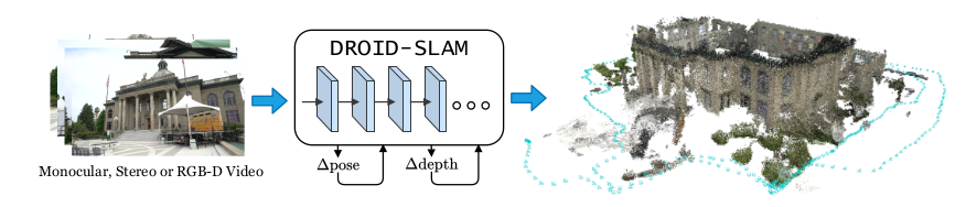
DROID-SLAM論文 Figure.1

DROID-SLAMはDeepLearningを用いたVSLAM(Visual Simultaneous Localization and Mapping)にRAFTで用いられた再帰的(recurrent)な処理を導入した研究です。

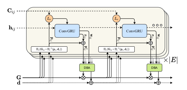
DROID-SLAM論文 Figure.2

上図はDROID-SLAMで用いられる再帰的(recurrent)な処理の概要です。DROID-SLAMの処理の大半はRAFTと共通するので下図と合わせて抑えておくと良いと思います。

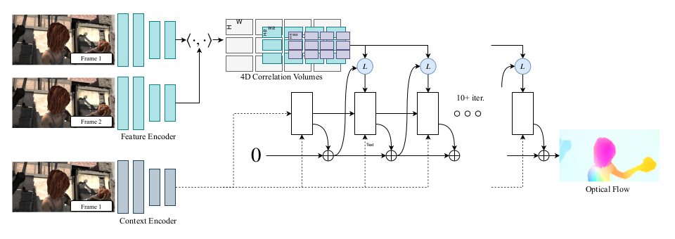
RAFT論文 Figure.1

数式に基づくDROID-SLAMの理解(4D Correlation)

DROID-SLAMの特徴量抽出と4D相関の計算処理はRAFTと同様に「Feature Extraction」、「Computing Correlation Pyramid」、「Correlation Lookup」の3つのプロセスで主に構成されます。「Feature Extraction」は基本的なCNNを用いて入力の1/8のサイズのFeature mapを構成する処理であり、一般的な処理であるので以下では「Computing Correlation Pyramid」と「Correlation Lookup」について数式に基づいて詳しく確認します。

Computing Correlation Pyramid

frame graph上のエッジ$(i, j) \in \mathcal{E}$のインデックス$i$と$j$のFeature map(Feature Extractionの出力に対応)を下記のように定義します。

\begin{align}
g_{\theta}(I_{i}), g_{\theta}(I_{j}) \in \mathbb{R}^{H \times W \times C}
\end{align}

このとき、$I_{i}$の位置$(u_{1}, v_{1})$と$I_{j}$の位置$(u_{2}, v_{2})$の相関を$C_{u_1 v_1 u_2 v_2}^{ij}$とおくと、$C_{u_1 v_1 u_2 v_2}^{ij}$は下記のように定義することができます。

\begin{align}
C_{u_1 v_1 u_2 v_2}^{ij} = \left< g_{\theta}(I_{i})_{u_1 v_1}, g_{\theta}(I_{j})_{u_2 v_2} \right>
\end{align}

Correlation Lookup

Correlation Lookupでは「4Dのうちの片方の画像に対応する2Dのそれぞれのピクセルについてもう片方の画像における位置$(x,y)$を指定し、その位置から半径$r$(実装上はユークリッドノルムではなく最大値ノルムを使用)の範囲の値をサンプリング」します。

\begin{align}
L_{r} : \mathbb{R}^{H \times W \times H \times W} \times \mathbb{R}^{H \times W \times 2} \mapsto \mathbb{R}^{H \times W \times (r+1)^{2}}
\end{align}

位置$\mathbf{u}=(x,y)$に関する最大値ノルム$||\mathbf{u}||_{\max}$は下記のように定義されます。

\begin{align}
||\mathbf{u}||_{\max} = ||\mathbf{u}||_{\infty} = \max\{ |x|, |y| \}
\end{align}

また、$(x, y)$は基本的に整数ではなく小数で得られるのでインデックスが整数のピクセル(grid)からサンプリングする際はバイリニア補間(bilinear interpolation)などが基本的に用いられます。

数式に基づくDROID-SLAMの理解(Update Operator)

Update Operatorの概略

DROID-SLAMではRAFTと同様に畳み込みGRU(Convolutional GRU)を用いて再帰的にカメラの位置や向きを取り扱う$\mathbf{G} \in SE(3)$や、画像のピクセルの深度を取り扱う$\mathbf{d} \in \mathbb{R}_{+}^{H \times W}$の推論を行います。

DROID-SLAM論文 Figure.2

DROID-SLAMのUpdate Operatorでは上図のような処理が行われます。$\mathbf{G} \in SE(3)$や$\mathbf{d} \in \mathbb{R}_{+}^{H \times W}$は下記のように値がUpdateされます。

\begin{align}
\mathbf{G}^{(k+1)} &= \exp{(\Delta \xi^{(k)} )} \circ \mathbf{G}^{(k)} \\
\mathbf{d}^{(k+1)} &= \Delta \mathbf{d}^{(k)} + \mathbf{d}^{(k)}
\end{align}

上記の$\Delta \xi^{(k)}$と$\Delta \mathbf{d}^{(k)}$をどのように得るかについて以下、確認を行います。

Correspondence

DROID-SLAMでは下記のような計算を行うことで$\mathbf{p}_{ij} \in \mathbb{R}^{H \times W \times 2}$を得ます。

\begin{align}
\mathbf{p}_{ij} &= \Pi_{c} (\mathbf{G}_{ij} \circ \Pi_{c}^{-1} (\mathbf{p}_{i}, \mathbf{d}_{i})) \in \mathbb{R}^{H \times W \times 2} \\
\mathbf{p}_{i} & \in \mathbb{R}^{H \times W \times 2} \\
\mathbf{G}_{ij} &= \mathbf{G}_{j} \circ \mathbf{G}_{i}^{-1}
\end{align}

上記の数式はエピポーラ幾何(Epipolar Geometry)に出てくる式に基づいて理解すれば良いです。$\Pi_{c}$はcamera model mappingです。$\Pi_{c}^{-1}$で3D化し$\Pi_{c}$で2D化するとざっくり抑えておけば当記事の範囲では十分だと思います。

DROID-SLAM論文 Figure.2

DROID-SLAMでは上図のように$\mathbf{G}$と$\mathbf{d}$に対しCorrespondence処理を適用することで$\mathbf{p}_{ij}$を取得し、再帰的な処理を行います。

Inputs

フレームグラフ$(\mathcal{V}, \mathcal{E})$のedgeの$(i, j) \in \mathcal{E}$が与えられたとき、4D相関の$C^{ij}$から相関の特徴量を取り出すにあたって$\mathbf{p}_{ij}$が用いられます。

$\mathbf{p}_{ij}$の周辺の相関の特徴量を用いることで類似する画像の領域の情報を取り扱えるようにネットワークを学習させることが可能になります。

Update

畳み込みGRU(Convolutional GRU)の演算では隠れ層の$\mathbf{h}^{(k+1)}$が生成されます。この生成された隠れ層に二つの畳み込み層を追加することで下記の二つの出力を作成します。

(1) a revision flow field $r_{ij} \in \mathbb{R}^{H \times W \times 2}$
(2) associated confidence map $w_{ij} \in \mathbb{R}_{+}^{H \times W \times 2}$

(1)の$r_{ij}$はcorrespondence fieldの$\mathbf{p}_{ij}$をUpdateする補正項であり、下記のような補正の計算を行います。

\begin{align}
\mathbf{p}_{ij}^{*} = \mathbf{p}_{ij} + r_{ij}
\end{align}

DBA(Dense Bundle Adjustment) Layer

DBA(Dense Bundle Adjustment) Layerでは下記のようなコスト関数$\mathbf{E}(\mathbf{G}', \mathbf{d}')$の最適化に基づいて前節で取り扱った$\Delta \xi^{(k)}$と$\Delta \mathbf{d}^{(k)}$の値の計算を行います。

\begin{align}
\mathbf{E}(\mathbf{G}', \mathbf{d}') &= \sum_{(i,j) \in \mathcal{E}} \left| \middle| \mathbf{p}_{ij}^{*} - \Pi_{c}(\mathbf{G}_{ij}' \circ \Pi_{c}^{-1}(\mathbf{p}_{i}, \mathbf{d}_{i}')) \middle| \right|_{\Sigma_{ij}}^{2} \\
\Sigma_{ij} &= \mathrm{diag} w_{ij}
\end{align}

ここで上記の式の$|| \cdot ||_{\Sigma}$はconfidence weightsの$w$によって重み付けされたエラー項(error term)のMahalanobis distanceです。
$\Delta \xi^{(k)}$と$\Delta \mathbf{d}^{(k)}$を得るにあたってはGauss-Newton algorithmが用いられます。

\begin{align}
\left(\begin{array}{cc} \mathbf{B} & E \\ \mathbf{E}^{\mathrm{T}} & \mathbf{C} \end{array} \right) \left(\begin{array}{c} \Delta \xi \\ \Delta \mathbf{d} \end{array} \right) = \left(\begin{array}{c} \mathbf{v} \\ \mathbf{w} \end{array} \right)
\end{align}

上記の式はシューア補行列(Schur complement)を用いることで効率的に解くことができ、下記のようなUpdateに用いる補正項の式が得られます。

\begin{align}
\Delta \xi &= \left[ \mathbf{B} - \mathbf{E}\mathbf{C}^{-1}\mathbf{E}^{\mathrm{T}} \right]^{-1} \left( \mathbf{v} - \mathbf{E}\mathbf{C}^{-1}w \right) \\
\Delta \mathbf{d} &= \mathbf{C}^{-1} \left( w - \mathbf{E}^{\mathrm{T}} \Delta \xi \right)
\end{align}

DROID-SLAMの学習と評価

DROID-SLAMの学習にあたってはTartanAir datasetが用いられています。学習の詳細については下記の表にまとめました。

コマンド名	動作
画像の解像度(resolution)	$384 \times 512$
フレーム数(frame clips)	$7$
バッチサイズ(batch size)	$4$
学習ステップ数(steps)	$250{,}000$
繰り返し数(iterations)	$15$
学習時間	$1$ week
用いたGPU	4 RTX-3090 GPUs

DROID-SLAMの評価については当記事ではTartanAir bonocular benchmarkとEuRoCの二つを確認します。

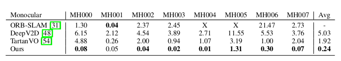
DROID-SLAM論文 Table.1

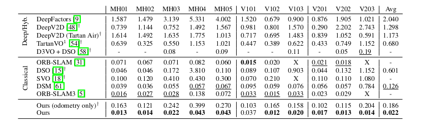
DROID-SLAM論文 Table.3

評価にあたっては絶対軌道誤差(ATE; Absolute Trajectory Error)が用いられています。

DROID-SLAMの実装

当節では下記のDROID-SLAMの実装について確認します。確認にあたってはsetup.pyでインストールするdroid_backendsやlietorchがうまく動かなかったので動作確認は行っていない点にご留意ください。

$ python train.py --datapath=<path to tartanair> --gpus=4 --lr=0.00025

README.mdに上記のような学習の実行コマンドが確認できます。

train.py

import torch.multiprocessing as mp

def train(gpu, args):
    ...
    
if __name__ == '__main__':
    ...
    mp.spawn(train, nprocs=args.gpus, args=(args,))

train.pyでは上記のようにtorch.multiprocessing.spawnを実行することでtrain関数内の処理が実行されます。よって以下ではtrain関数の内部の内部の処理について確認を行います。

DROID-SLAMのmodel

train.py

import sys
sys.path.append('droid_slam')

...

from droid_net import DroidNet
from torch.nn.parallel import DistributedDataParallel as DDP

...

def train(gpu, args):
    """ Test to make sure project transform correctly maps points """

    # coordinate multiple GPUs
    setup_ddp(gpu, args)
    rng = np.random.default_rng(12345)

    N = args.n_frames
    model = DroidNet()
    model.cuda()
    model.train()

    model = DDP(model, device_ids=[gpu], find_unused_parameters=False)

    if args.ckpt is not None:
        model.load_state_dict(torch.load(args.ckpt))
        
    ...
    
    # fetch optimizer
    optimizer = torch.optim.Adam(model.parameters(), lr=args.lr, weight_decay=1e-5)
    
    ...
    
    while should_keep_training:
        for i_batch, item in enumerate(train_loader):
            ...
            while r < args.restart_prob:
                r = rng.random()
                
                intrinsics0 = intrinsics / 8.0
                poses_est, disps_est, residuals = model(Gs, images, disp0, intrinsics0, 
                    graph, num_steps=args.iters, fixedp=2)

                geo_loss, geo_metrics = losses.geodesic_loss(Ps, poses_est, graph, do_scale=False)
                res_loss, res_metrics = losses.residual_loss(residuals)
                flo_loss, flo_metrics = losses.flow_loss(Ps, disps, poses_est, disps_est, intrinsics, graph)

                loss = args.w1 * geo_loss + args.w2 * res_loss + args.w3 * flo_loss
                loss.backward()
                
    ...

上記がDROID-SLAMのmodelに関連する実装です。上記よりdroid_slam/droid_net.pyのDroidNetクラスにmodelの処理が基本的には書かれていることが確認できます。

droid_slam/droid_net.py

lass DroidNet(nn.Module):
    def __init__(self):
        super(DroidNet, self).__init__()
        self.fnet = BasicEncoder(output_dim=128, norm_fn='instance')
        self.cnet = BasicEncoder(output_dim=256, norm_fn='none')
        self.update = UpdateModule()


    def extract_features(self, images):
        """ run feeature extraction networks """

        # normalize images
        images = images[:, :, [2,1,0]] / 255.0
        mean = torch.as_tensor([0.485, 0.456, 0.406], device=images.device)
        std = torch.as_tensor([0.229, 0.224, 0.225], device=images.device)
        images = images.sub_(mean[:, None, None]).div_(std[:, None, None])

        fmaps = self.fnet(images)
        net = self.cnet(images)
        
        net, inp = net.split([128,128], dim=2)
        net = torch.tanh(net)
        inp = torch.relu(inp)
        return fmaps, net, inp


    def forward(self, Gs, images, disps, intrinsics, graph=None, num_steps=12, fixedp=2):
        """ Estimates SE3 or Sim3 between pair of frames """

        u = keyframe_indicies(graph)
        ii, jj, kk = graph_to_edge_list(graph)

        ii = ii.to(device=images.device, dtype=torch.long)
        jj = jj.to(device=images.device, dtype=torch.long)

        fmaps, net, inp = self.extract_features(images)
        net, inp = net[:,ii], inp[:,ii]
        corr_fn = CorrBlock(fmaps[:,ii], fmaps[:,jj], num_levels=4, radius=3)

        ht, wd = images.shape[-2:]
        coords0 = pops.coords_grid(ht//8, wd//8, device=images.device)
        
        coords1, _ = pops.projective_transform(Gs, disps, intrinsics, ii, jj)
        target = coords1.clone()

        Gs_list, disp_list, residual_list = [], [], []
        for step in range(num_steps):
            Gs = Gs.detach()
            disps = disps.detach()
            coords1 = coords1.detach()
            target = target.detach()

            # extract motion features
            corr = corr_fn(coords1)
            resd = target - coords1
            flow = coords1 - coords0

            motion = torch.cat([flow, resd], dim=-1)
            motion = motion.permute(0,1,4,2,3).clamp(-64.0, 64.0)

            net, delta, weight, eta, upmask = \
                self.update(net, inp, corr, motion, ii, jj)

            target = coords1 + delta

            for i in range(2):
                Gs, disps = BA(target, weight, eta, Gs, disps, intrinsics, ii, jj, fixedp=2)

            coords1, valid_mask = pops.projective_transform(Gs, disps, intrinsics, ii, jj)
            residual = (target - coords1)

            Gs_list.append(Gs)
            disp_list.append(upsample_disp(disps, upmask))
            residual_list.append(valid_mask * residual)


        return Gs_list, disp_list, residual_list

Bundle Adjustmentの処理

droid_slam/droid_net.py

from geom.ba import BA

...

class DroidNet(nn.Module):

    ...

    def forward(self, Gs, images, disps, intrinsics, graph=None, num_steps=12, fixedp=2):
        ...
        for step in range(num_steps):
            ...
            for i in range(2):
                Gs, disps = BA(target, weight, eta, Gs, disps, intrinsics, ii, jj, fixedp=2)
     ...

Bundle Adjustmentの処理は上記のようにDroidNetクラスのBAを用いて行われます。以下geom/ba.pyのBAクラスを確認します。

geom/ba.py

def BA(target, weight, eta, poses, disps, intrinsics, ii, jj, fixedp=1, rig=1):
    """ Full Bundle Adjustment """

    B, P, ht, wd = disps.shape
    N = ii.shape[0]
    D = poses.manifold_dim

    ### 1: commpute jacobians and residuals ###
    coords, valid, (Ji, Jj, Jz) = pops.projective_transform(
        poses, disps, intrinsics, ii, jj, jacobian=True)

    r = (target - coords).view(B, N, -1, 1)
    w = .001 * (valid * weight).view(B, N, -1, 1)

    ### 2: construct linear system ###
    Ji = Ji.reshape(B, N, -1, D)
    Jj = Jj.reshape(B, N, -1, D)
    wJiT = (w * Ji).transpose(2,3)
    wJjT = (w * Jj).transpose(2,3)

    Jz = Jz.reshape(B, N, ht*wd, -1)

    Hii = torch.matmul(wJiT, Ji)
    Hij = torch.matmul(wJiT, Jj)
    Hji = torch.matmul(wJjT, Ji)
    Hjj = torch.matmul(wJjT, Jj)

    vi = torch.matmul(wJiT, r).squeeze(-1)
    vj = torch.matmul(wJjT, r).squeeze(-1)

    Ei = (wJiT.view(B,N,D,ht*wd,-1) * Jz[:,:,None]).sum(dim=-1)
    Ej = (wJjT.view(B,N,D,ht*wd,-1) * Jz[:,:,None]).sum(dim=-1)

    w = w.view(B, N, ht*wd, -1)
    r = r.view(B, N, ht*wd, -1)
    wk = torch.sum(w*r*Jz, dim=-1)
    Ck = torch.sum(w*Jz*Jz, dim=-1)

    kx, kk = torch.unique(ii, return_inverse=True)
    M = kx.shape[0]

    # only optimize keyframe poses
    P = P // rig - fixedp
    ii = ii // rig - fixedp
    jj = jj // rig - fixedp

    H = safe_scatter_add_mat(Hii, ii, ii, P, P) + \
        safe_scatter_add_mat(Hij, ii, jj, P, P) + \
        safe_scatter_add_mat(Hji, jj, ii, P, P) + \
        safe_scatter_add_mat(Hjj, jj, jj, P, P)

    E = safe_scatter_add_mat(Ei, ii, kk, P, M) + \
        safe_scatter_add_mat(Ej, jj, kk, P, M)

    v = safe_scatter_add_vec(vi, ii, P) + \
        safe_scatter_add_vec(vj, jj, P)

    C = safe_scatter_add_vec(Ck, kk, M)
    w = safe_scatter_add_vec(wk, kk, M)

    C = C + eta.view(*C.shape) + 1e-7

    H = H.view(B, P, P, D, D)
    E = E.view(B, P, M, D, ht*wd)

    ### 3: solve the system ###
    dx, dz = schur_solve(H, E, C, v, w)
    
    ### 4: apply retraction ###
    poses = pose_retr(poses, dx, torch.arange(P) + fixedp)
    disps = disp_retr(disps, dz.view(B,-1,ht,wd), kx)

    disps = torch.where(disps > 10, torch.zeros_like(disps), disps)
    disps = disps.clamp(min=0.0)

    return poses, disps

DROID-SLAMのloss

train.py

...

from geom.losses import geodesic_loss, residual_loss, flow_loss

...

def train(gpu, args):

    ...

    while should_keep_training:
        for i_batch, item in enumerate(train_loader):

            ...

            while r < args.restart_prob:
                r = rng.random()
                
                intrinsics0 = intrinsics / 8.0
                poses_est, disps_est, residuals = model(Gs, images, disp0, intrinsics0, 
                    graph, num_steps=args.iters, fixedp=2)

                geo_loss, geo_metrics = losses.geodesic_loss(Ps, poses_est, graph, do_scale=False)
                res_loss, res_metrics = losses.residual_loss(residuals)
                flo_loss, flo_metrics = losses.flow_loss(Ps, disps, poses_est, disps_est, intrinsics, graph)

                loss = args.w1 * geo_loss + args.w2 * res_loss + args.w3 * flo_loss
                loss.backward()

    ...

上記よりDROID-SLAMのlossはgeom/losses.pyに実装されていることが確認できます。

geom/losses.py

def geodesic_loss(Ps, Gs, graph, gamma=0.9, do_scale=True):
    """ Loss function for training network """

    # relative pose
    ii, jj, kk = graph_to_edge_list(graph)
    dP = Ps[:,jj] * Ps[:,ii].inv()

    n = len(Gs)
    geodesic_loss = 0.0

    for i in range(n):
        w = gamma ** (n - i - 1)
        dG = Gs[i][:,jj] * Gs[i][:,ii].inv()

        if do_scale:
            s = fit_scale(dP, dG)
            dG = dG.scale(s[:,None])
        
        # pose error
        d = (dG * dP.inv()).log()

        if isinstance(dG, SE3):
            tau, phi = d.split([3,3], dim=-1)
            geodesic_loss += w * (
                tau.norm(dim=-1).mean() + 
                phi.norm(dim=-1).mean())

        elif isinstance(dG, Sim3):
            tau, phi, sig = d.split([3,3,1], dim=-1)
            geodesic_loss += w * (
                tau.norm(dim=-1).mean() + 
                phi.norm(dim=-1).mean() + 
                0.05 * sig.norm(dim=-1).mean())
            
        dE = Sim3(dG * dP.inv()).detach()
        r_err, t_err, s_err = pose_metrics(dE)

    metrics = {
        'rot_error': r_err.mean().item(),
        'tr_error': t_err.mean().item(),
        'bad_rot': (r_err < .1).float().mean().item(),
        'bad_tr': (t_err < .01).float().mean().item(),
    }

    return geodesic_loss, metrics


def residual_loss(residuals, gamma=0.9):
    """ loss on system residuals """
    residual_loss = 0.0
    n = len(residuals)

    for i in range(n):
        w = gamma ** (n - i - 1)
        residual_loss += w * residuals[i].abs().mean()

    return residual_loss, {'residual': residual_loss.item()}


def flow_loss(Ps, disps, poses_est, disps_est, intrinsics, graph, gamma=0.9):
    """ optical flow loss """

    N = Ps.shape[1]
    graph = OrderedDict()
    for i in range(N):
        graph[i] = [j for j in range(N) if abs(i-j)==1]

    ii, jj, kk = graph_to_edge_list(graph)
    coords0, val0 = projective_transform(Ps, disps, intrinsics, ii, jj)
    val0 = val0 * (disps[:,ii] > 0).float().unsqueeze(dim=-1)

    n = len(poses_est)
    flow_loss = 0.0

    for i in range(n):
        w = gamma ** (n - i - 1)
        coords1, val1 = projective_transform(poses_est[i], disps_est[i], intrinsics, ii, jj)

        v = (val0 * val1).squeeze(dim=-1)
        epe = v * (coords1 - coords0).norm(dim=-1)
        flow_loss += w * epe.mean()

    epe = epe.reshape(-1)[v.reshape(-1) > 0.5]
    metrics = {
        'f_error': epe.mean().item(),
        '1px': (epe<1.0).float().mean().item(),
    }

    return flow_loss, metrics