scipy.spatial.cKDTreeとquery_ball_pointを用いた近傍探索

scipy.spatial.cKDTreeやscipy.spatial.cKDTree.query_ball_pointを用いた近傍探索は点群処理の前処理で使われることがあるので以下簡単に確認を行います。

サンプルコード

下記のようなコードを動かすことでscipy.spatial.cKDTreeやscipy.spatial.cKDTree.query_ball_pointを用いた近傍探索を行うことができます。

import matplotlib.pyplot as plt
import numpy as np
from scipy import spatial

x, y = np.mgrid[1:6, 1:6]
points = np.c_[x.ravel(), y.ravel()]

tree = spatial.cKDTree(points)

points = np.asarray(points)
plt.plot(points[:,0], points[:,1], '.')

for results in tree.query_ball_point(([2, 3], [5, 5]), 1):
    nearby_points = points[results]
    plt.plot(nearby_points[:,0], nearby_points[:,1], 'o')

plt.margins(0.1, 0.1)
plt.savefig("cKD-Tree.png")

・実行結果

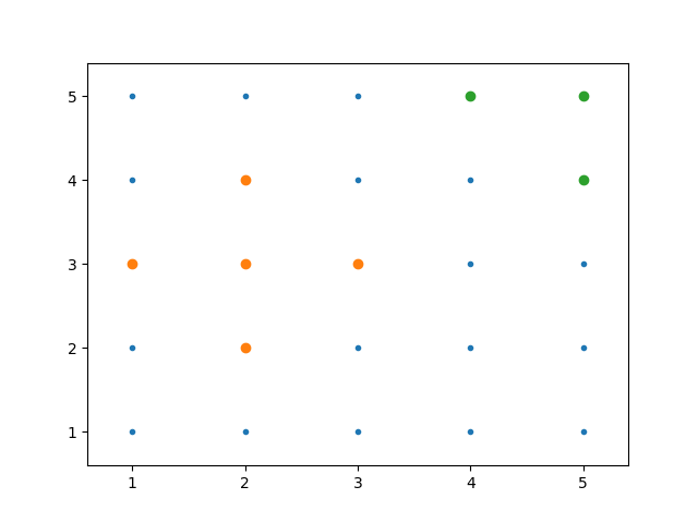
実行結果の理解にあたっては「(2,3)の半径1以内の点である(2,2)、(1,3)、(2,3)、(3,3)、(2,4)」がオレンジ、「(5,5)の半径1以内の点である(4,5)、(5,4)、(5,5)」が緑で表されたことに着目すると良いです。

サンプルコードの理解

以下、前節で取り扱ったコードの詳細について確認を行います。

import matplotlib.pyplot as plt
import numpy as np
from scipy import spatial

x, y = np.mgrid[1:6, 1:6]
points = np.c_[x.ravel(), y.ravel()]

print(points)

tree = spatial.cKDTree(points)
nearby_points = tree.query_ball_point([2, 2], 1)

print(nearby_points)
print(points[nearby_points])

・実行結果

[[1 1]
 [1 2]
 [1 3]
 [1 4]
 [1 5]
 [2 1]
 [2 2]
 [2 3]
 [2 4]
 [2 5]
 [3 1]
 [3 2]
 [3 3]
 [3 4]
 [3 5]
 [4 1]
 [4 2]
 [4 3]
 [4 4]
 [4 5]
 [5 1]
 [5 2]
 [5 3]
 [5 4]
 [5 5]]
[1, 7, 6, 5, 11]
[[1 2]
 [2 3]
 [2 2]
 [2 1]
 [3 2]]

上記より、scipy.spatial.cKDTree.query_ball_pointは(2,2)の半径1以内の点を探索し、pointsの点のインデックスの形式で出力を行っていることが確認できます。ここでは二次元を取り扱いましたが、三次元の点群を取り扱うなども可能です。

・参考