Pythonプログラミング：ウィキペディアのデータを使ってword2vecをしてみる｛4. モデル応用編｝

はじめに

4本立ての記事、4本目（最後）です。

1. データ取得＆前処理編
2. モデル作成編
3. モデル利用編
4. モデル応用編　★本稿

本稿で紹介すること

• word2vecモデルの応用

以下のリンク、5つ目に掲載されたCodeを見本とし、筆者が作ったword2vecモデルを使って試行しました！

word2vec
Word2vec Tutorial
Deep learning with word2vec and gensim
米googleの研究者が開発したWord2Vecで自然言語処理(独自データ)
【Python】word2vecとクラスタリングでwikiコーパスを使って遊ぶ

本稿で紹介しないこと

• word2vecの仕組み
• Pythonライブラリの使い方
  • gensim　※単語の分散表現（単語ベクトル）を実現するPythonライブラリ
• word2vecモデルの作成
• word2vecモデルの利用

【まとめ】自然言語処理における単語分散表現（単語ベクトル）と文書分散表現（文書ベクトル）
word2vec（Skip-Gram Model）の仕組みを恐らく日本一簡潔にまとめてみたつもり
【Python】Word2Vecの使い方
gensim/word2vec.py
gensim: models.word2vec – Word2vec embeddings

モデル応用編

モデル利用に続き、Windowsで進めます。

word2vecモデルの応用

いくつかの単語をピックアップし、各単語の分散表現（単語ベクトル）を使ってクラスタリングをします。

まず、事前に作成（学習）したword2vecモデルを読み込みます。

analyzeWiki_Word2Vec3

from gensim.models import Word2Vec

model = Word2Vec.load(r'..\result\jawiki_word2vec_sz200_wndw10.model')
wv = model.wv

そして、各単語の分散表現を取得します。
分散表現を取得する際、KeyErrorが発生する可能性を考慮する必要がありますが、今回は割愛します。（本来なら、Try～Exceptの構文を用いるところかと。）

analyzeWiki_Word2Vec3

from scipy.cluster.hierarchy import linkage, dendrogram
import matplotlib.pyplot as plt
%matplotlib inline

words = ["東京", "神奈川", "千葉", "埼玉", "日本", "アメリカ", "ドイツ", "セダン", "ワゴン", "トラック", "自動車", "飛行機", "船舶", "列車"]
vectors = [model[word] for word in words]

#日本語フォントの指定
import matplotlib.pyplot as plt
plt.rcParams["font.family"] = 'Yu Gothic'

以下、モデル応用のCodeを紹介。

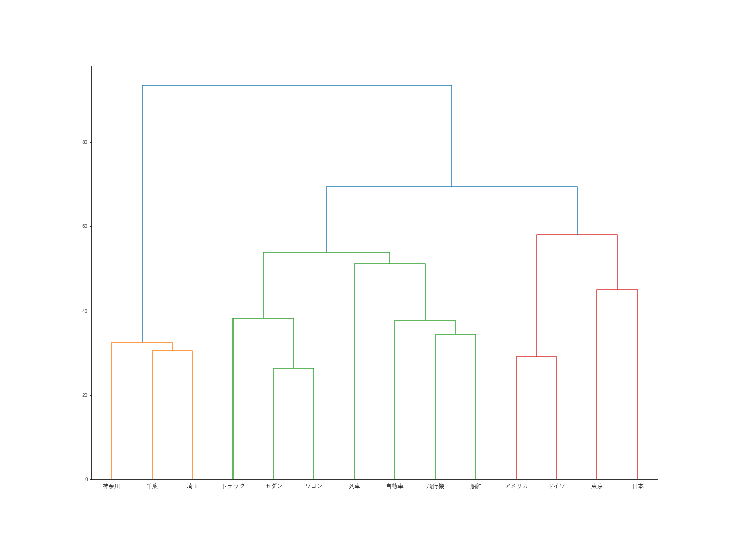
階層型クラスタリング（距離関数：ウォード法）

”日本”が”東京”とくっついてしまいました。その他は、まぁ期待通りという感じです。

analyzeWiki_Word2Vec3

l = linkage(vectors, method="ward")
plt.figure(figsize=(20, 15))
dendrogram(l, labels=words)
plt.savefig("../result/word_clustering_dendrogram1.png")

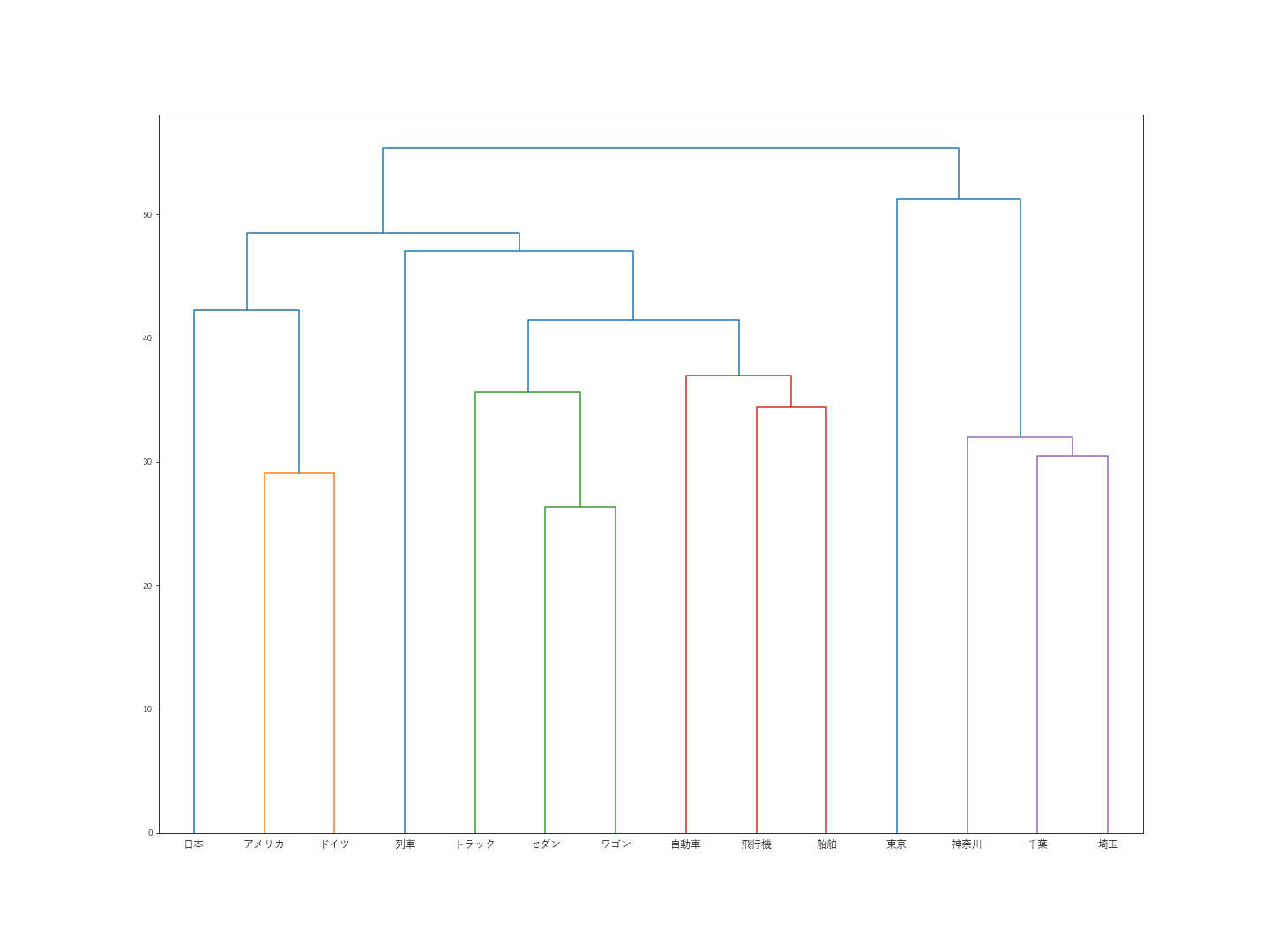
階層型クラスタリング（距離関数：群平均法）

”日本”が”東京”とくっついてしまったのは変わらず。その他だと、”列車”がなぜか遠い場所へ行ってしまいました。

analyzeWiki_Word2Vec3

l = linkage(vectors, method="average")
plt.figure(figsize=(20, 15))
dendrogram(l, labels=words)
plt.savefig("../result/word_clustering_dendrogram2.png")

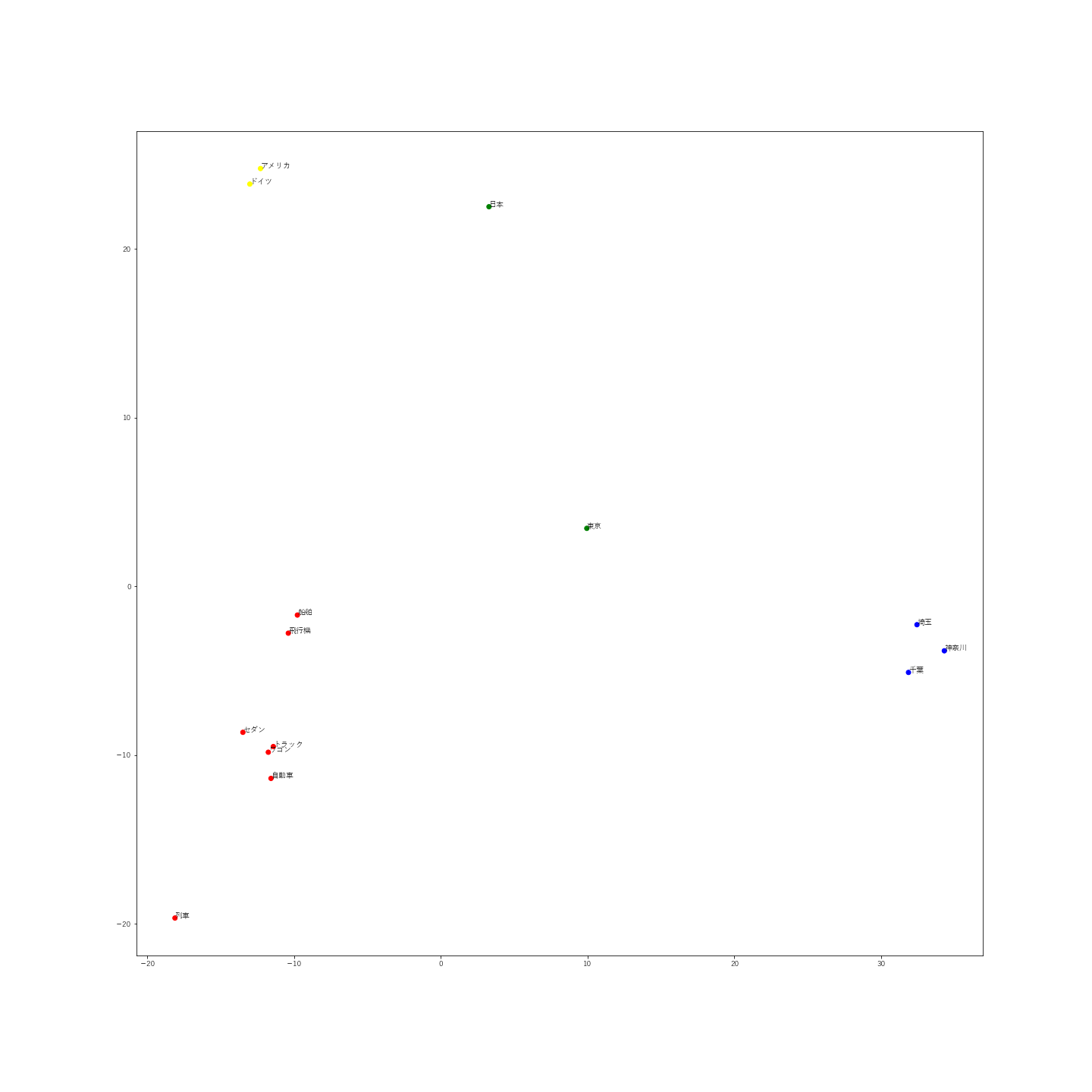
非階層型クラスタリング

階層型クラスタリングでも想定外の分類だった、”東京”が宙ぶらりんな感じで位置しています。
この結果を見ると、「都市」のクラスタではなく、「国」のクラスタ（特に、最も近い”日本”）に属するのもやむなしかな、と納得してしまいました。

analyzeWiki_Word2Vec3

from sklearn.cluster import KMeans
from sklearn.decomposition import PCA
import pandas as pd
import matplotlib.pyplot as plt
from collections import defaultdict

kmeans_model = KMeans(n_clusters=4, verbose=1, random_state=0).fit(vectors)
cluster_labels = kmeans_model.labels_
cluster_to_words = defaultdict(list)
for cluster_id, word in zip(cluster_labels, words):
    cluster_to_words[cluster_id].append(word)

print(cluster_labels)
for l, w in cluster_to_words.items():
    print('=====')
    print(l)
    print('-----')
    print(w)
    print('=====')

df = pd.DataFrame(vectors)
df["word"] = words
df["cluster"] = cluster_labels

#PCAで2次元に圧縮
pca = PCA(n_components=2)
pca.fit(df.iloc[:, :-2])
feature = pca.transform(df.iloc[:, :-2])

#日本語フォントの指定
import matplotlib.pyplot as plt
plt.rcParams["font.family"] = 'Yu Gothic'

#散布図プロット
color = {0:"green", 1:"red", 2:"yellow", 3:"blue"}
colors = [color[x] for x in cluster_labels]
plt.figure(figsize=(20, 20))
for x, y, name in zip(feature[:, 0], feature[:, 1], df.iloc[:, -2]):
    plt.text(x, y, name)
plt.scatter(feature[:, 0], feature[:, 1], color=colors)
plt.savefig("../result/word_clustering_scatter.png")
plt.show()

まとめ

ウィキペディアの前処理済みデータから作成済みの、word2vecモデルを応用する方法を紹介。