Source
Introduction
This paper propose a method which is able to learn character interactions that involve multiple contacts between the body and
an object, another character and the environment, from a rich, unstructured motion capture database.
The author introduce two main novelties; one is a feature called local motion phase that enables the synthesize of high quality movements, and another is a generative model which can convert an abstract, high-level user control signal into a wide variation of sharp signals that can be mapped to realistic character movements.
Algorithm
Overview
The system consists of a motion prediction network and a gating network (Fig. 2).
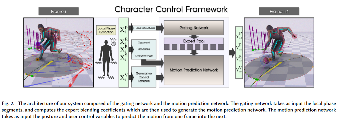
System Inputs and Outputs
Inputs
The system is a time-series model that predicts the state variables of the character, the ball etc. in the next frame $i+1$ given those in the current frame $i$. All features live in a time series window $\tau_{-1s}^{1s}$ within which data of 13 uniformly-sampled points (6 each in the future and past 1s window, and one for the current frame) are collected.
The complete input vector $X_i$ at frame $i$ consists of five components $X_i =$ {$X_i^S ,X_i^V ,X_i^F ,X_i^R ,X_i^P$} where each item is described below.
-
Character State $X_i^S =$ {$p_i ,r_i ,v_i$} represents the state of the character at the current frame $i$. It consists of bone positions $p_i$, bone rotations $r_i$ and bone velocities $v_i$, for a total of 26 different bones.
-
Control Variables $X_i^V =$ {$T_i^p ,T_i^r ,T_i^v ,I_i^p ,I_i^m ,A_i$} are the variables used to guide the character to conduct various basketball movements.
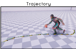
– Root Trajectory T for controlling the character locomotion, with horizontal path of trajectory positions $T_i^p$, trajectory directions $T_i^r$ and trajectory velocities $T_i^v$.
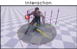
– Interaction Vectors I, a set of 3D pivot vectors $I_i^p$ and its derivative $I_i^m$ around the character, that together define the dribbling direction, height and speed to direct a wide range of dynamic ball interaction movements and maneuvers.
– Action Variables $A_i$ which consist of four actions that are defined as A ={Idle,Move,Control,Hold}, where each of them is between 0 and 1. -
Conditioning Features $X_i^F =$ {$B_i^p,B_i^v ,B_i^w ,C_i$}
– Ball Movement $B$. The past movement of the ball of positions $\hat{B_i^p}$ and velocities $\hat{B_i^v}$ is used to guide the prediction for next frame. In addition, ball control weights $B_i^w$ are given as input to the network, which were used to transform the original ball parameters from $B_i$ to $\hat{B_i}$ in order to learn the ball movement only within a control radius around the character.
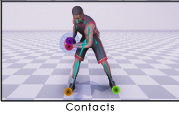
– Contact Information $C$. Conditions the generated motion on the contacts $C$ for feet, hands and ball that appeared during the past to stabilize the movements.
-
Opponent Information $X_i^R =$ {$w_i, d_i, g_i^p, g_i^r, g_i^v$} are the variables that describe the state of the opponent character with respect to the user character.
– $w_i = 1$ if the opponent is within 5 meter radius, 0 otherwise,
– $g_i^p, g_i^r, g_i^v$ are 2D vectors between position samples of the user and opponent trajectories, as well the direction and velocity of the opponent trajectory. These are weighted by $w_i$ for cases where the opponent is out of range or unavailable.
– $d_i$ are the distance pairs within 5m radius between the corresponding B =26 joints of the two characters at current frame $i$.

-
Local Motion Phases $X_i^P = Θ_i$ are each represented by 2D phase vectors of changing amplitude for the 5 key bones; feet, hands and ball.
Outputs
The output vector $Y_{i+1} =$ {$Y_{i+1}^S, Y_{i+1}^V, Y_{i+1}^F, Y_{i+1}^P$} for the next frame $i+1$ is computed by the motion prediction network, and consists of the following four components.
- Character State $Y_{i+1}^S$ is pose and velocity of the character at next frame $i+1$.
-
Future Control Variables $Y_{i+1}^V$. During runtime, these features are blended with the given user-guided control signals and fed into the input in the next frame, such that the character produces plausible motion while following the user instruction:
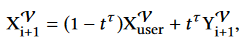
– $X_{user}^V$ are the control signals produced from the user inputs
– $t$ ranges from 0 to 1 as the trajectory gets further into the future
– τ is an additional bias that controls the responsiveness of the character. - Conditioning Features $Y_{i+1}^F =$ {$\hat{B_{i+1}^p}, \hat{B_{i+1}^r}, \hat{B_{i+1}^v}, B_{i+1}^w, C_{i+1}$} are computed for the next frame $i+1$. The output also includes the delta ball rotation $\hat{B_{i+1}^r}$, which is used to update the orientation of the ball in the next frame.
-
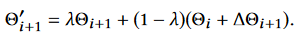
Local Motion Phases Updates $X_{i+1}^P =$ {$\theta_{i+1}, ∆\theta_{i+1}$}, which contain the phase vectors for the 5 key bones $\theta_{i+1}$ and their updates $∆\theta_{i+1}$ for the 5 key bones. All phases can be updated asynchronously and independently, and the new updated phase vectors $\theta'_{i+1}$ is calculated as:
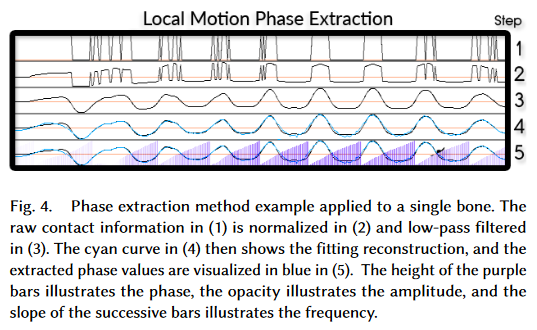
Local Motion Phase
The local motion phase allows the system to learn to align the local limb movements individually, while also integrating their movements to produce realistic full-body behavior.
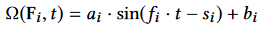
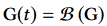
The local phase is computed from the motion capture data by fitting a sinusoidal function to a filter block function $G(t)$that represents the contact between the bone and the object/environment.
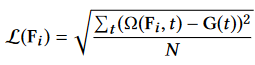
At every frame $i$, we minimizes the RMSE loss inside a windows of $N$ frames centered at frame $i$:
$G(t)$ is computed by first normalizing the original block function in a window $W$ of 60 frames (1 second) centered at frame $j$:
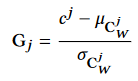
where $c_j$ is the original block function value, and $\mu_{C_w^j}$ and $\alpha_{C_w^j}$ are the mean and standard deviation of contacts within that window, and then applying a Butterworth low-pass filter to the entire domain:
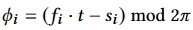
By minimizing the loss, a 1D phase value is calculated as:
We can then obtain 2D vectors $P$ for the bones, containing information about the timing and speed of the movement, and are fed into the gating neural network as features.
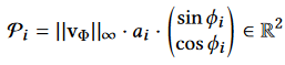
where $a_i$ is the optimized amplitude parameter, $||v_{\phi}||_{\infty}$ is the maximum bone velocity magnitude and $\Phi$ is the frequency-based frame window.
Generative Control Model
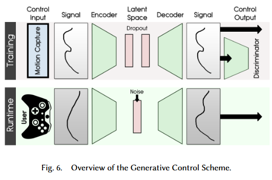
The generative control model has three components:
- An encoder $E$, which first takes a smoothed trajectory produced by blending the user gamepad input signal and the autoregressive control signal
from the previous time step and encodes it into a latent code. - A decoder $G$ that produces the control signal from the latent code.
- A discriminator $D$ that distinguishes the generated control signal from the ground truth control signal (outputs a probability between 0 and 1).
The model is trained similar to a normal GAN, where the control variable $X^V$ is passed into the encoder and reconstructed by the decoder. The reconstructed signal then gets evaluated by the discriminator.
During runtime, $X^V$ is computed by blending $Y^V$ in the previous cycle with the user input signals and passed into the encoder. The latent value is mixed with a random noise sampled from a Gaussian, and thus a control signal recovered by the decoder will be containing valid variance which is very hard to be hand-coded from gamepad input. In order to manage the controllability of the character, they sample noise vectors from different random seed and use them as style variables. The animator can pick them as the behavior style of each character.
Training
The training is done by first normalizing the input and the output of the full dataset by their mean and standard deviation, pretraining the generative control model and then training the main network composed of the gating network and motion prediction network in an end-to-end fashion.
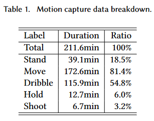
The complete breakdown of the training dataset can be seen below:
Result
Evaluation Metrics
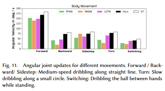
Body movement
Calculated as the sum of the absolute angle updates of all the joints per frame. The proposed method outperforms existing algorithms, especially for movements where the data samples are sparse.
Contact Accuracy
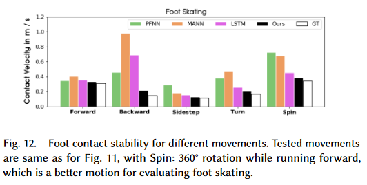
The amount of foot skating is calculated by summing the horizontal movements of the feet when their height and vertical velocity are below thresholds.
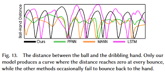
They also compute dribble accuracy where an accurate dribbling means the distance between the hand and the ball needs to go zero for every bounce of the ball.
Responsiveness
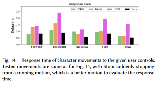
Measured as the average time required for completing tasks since the user input signal was given (e.g. reach the target speed and orientation).
Other Takeaways
- System is able to synthesize combination of movements that is not present in the training dataset (e.g. behind the back dribble while walking backwards).
- While the system can learn one-on-one movements from the training data, it is not always realistic and will require future research.
- Can learn quadruped motion control.
- Can learn object interaction.
Conclusion
The proposed method improves the control of character movements to a more realistic level. However, there are still many obstacles that needs to be tackled before it can be implemented for real game usage. For example, while it is impressive that new moves discovered by the network, it may not be allowed in an actual basketball game (e.g. running and holding the ball at the same time). How the movement of the character (during both training and runtime) will be affected if multiple bodies (players) are present is also another challenge that needs to be further investigated.