金融界隈で定量的な分析やデータサイエンスをやっている9uantです.
twitterもやってるので,興味ある方はぜひフォローしていただけると!
1. 経済データの「レジーム」
ITバブル崩壊やリーマンショックなど、経済に急激で大きな変化が生じた時とき、背景で根本的に何らかの状態が変化してしまっていると考えられる場合がある。このような根本的な状態の変化モデルを「レジームスイッチングモデル」という。
変化した状態が観測不可能な場合、レジームスイッチをモデル化することは難しそうである。しかし、レジームの確率分布をパラメータ付きで与え、レジーム間の遷移をマルコフ連鎖と捉えることで、モデル化が可能になる。MCMCによって尤度を最大化するパラメータ(正規分布の平均・標準偏差、レジームの遷移確率)を求めることができるのである。
2. マルコフ・スイッチングモデルの解説
レジーム付き線形回帰
以下の線形回帰モデルのレジームスイッチングモデルを考える。
\begin{eqnarray}
y\left( t \right) &=& x\left( t \right)\beta + \epsilon\left( t \right)\\
\epsilon\left( t \right)&\sim& N\left(0,\sigma^2\right)
\end{eqnarray}
各時刻$t$における第$1$〜第$n$レジームを以下のように表す。
\begin{eqnarray}
I\left(t\right) \in { 1,2,\cdots ,n}
\end{eqnarray}
レジームを観測できる場合、回帰式はレジームを添え字として以下のように表される。
\begin{eqnarray}
y\left( t \right) &=& x\left( t \right)\beta_{I\left( t\right)} + \epsilon\left( t \right)\\
\epsilon\left( t \right)&\sim& N\left(0,\sigma^2_{I\left( t\right)}\right)
\end{eqnarray}
このとき、$y\left( t\right)$は、平均$x\left( t \right)\beta_{I\left( t\right)}$、分散$\sigma^2_{I\left( t\right)}$の正規分布に従う。対数尤度を最大化する最尤法を適用する。すなわち、以下の尤度関数を最大とするパラメータを求める。
\begin{eqnarray}
\ln{\mathcal{L}}&=&\sum_{t=1}^{T}\ln{\{f\left( y\left( t\right)|I\left( t\right)\right)\} }\\
f\left( y\left( t\right)|I\left( t\right)\right)&=&\frac{1}{\sqrt{2\pi\sigma^2_{I\left( t\right)}}}\exp\left( -\frac{\{y\left( t\right)-x\left( t\right)\beta_{I\left( t \right)}\}^2}{2\sigma^2_{I\left( t\right)}}\right)
\end{eqnarray}
レジームを直接観測できない場合、$I\left( t\right)$も過去の履歴の条件付き確率分布に従うと考える。
時点$t$までに得られる情報を$\mathcal{F}\left( t\right)$とする。
$f\left( t\right)$は$\mathcal{F}\left( t\right)$に条件付けられないことに注意する。
\begin{eqnarray}
f\left( y\left( t\right) | \mathcal{F\left( t-1\right)}\right) &=& \sum_{I\left( t\right)=1}^{n}f\left( y\left( t\right),I\left( t\right) |\mathcal{F}\left( t-1\right)\right)\\
&=& \sum_{I\left( t\right)=1}^{n}f\left( y\left( t\right)|I\left( t\right),\mathcal{F}\left( t-1\right)\right)f\left( I\left( t\right)|\mathcal{F}\left( t-1\right)\right)\\
&=& \sum_{I\left( t\right)=1}^{n}\frac{1}{\sqrt{2\pi\sigma^2_{I\left( t\right)}}}\exp\left( -\frac{\{y\left( t\right)-x\left( t\right)\beta_{I\left( t \right)}\}^2}{2\sigma^2_{I\left( t\right)}}\right)
f\left( I\left( t\right)|\mathcal{F}\left( t-1\right)\right)
\end{eqnarray}
したがって、最大化する対数尤度は以下の通りである。
\begin{eqnarray}
\ln{\mathcal{L}}&=&\sum_{t=1}^{T}\ln{\left\{\sum_{I\left( t\right)=1}^{n}f\left( y\left( t\right)|I\left( t\right),\mathcal{F}\left( t-1\right)\right)f\left( I\left( t\right)|\mathcal{F}\left( t-1\right)\right)\right\} }\\

f\left( y\left( t\right)|I\left( t\right),\mathcal{F}\left( t-1\right)\right)&=&\frac{1}{\sqrt{2\pi\sigma^2_{I\left( t\right)}}}\exp\left( -\frac{\{y\left( t\right)-x\left( t\right)\beta_{I\left( t \right)}\}^2}{2\sigma^2_{I\left( t\right)}}\right)
\end{eqnarray}
マルコフ連鎖
$f\left( I\left( t\right)|\mathcal{F}\left( t-1\right)\right)$を与えることで、$y\left( t\right)$の確率分布が定まる。$I\left( t\right)$が1次のマルコフ性を満たすと仮定する。
\begin{eqnarray}
P\left( I\left( t\right)=i|\mathcal{F}\left( t-1\right)\right)
&=&\sum_{j=1}^{n}P\left( I\left( t\right)=i,I\left( t-1\right)=j|\mathcal{F}\left( t-1\right)\right)\\
&=&\sum_{j=1}^{n}P\left( I\left( t\right)=i|I\left( t-1\right)=j\right)P\left( I\left( t-1\right)=j|\mathcal{F}\left( t-1\right)\right)
\end{eqnarray}
状態jから状態iへの遷移確率$P\left( I\left( t\right)=i|I\left( t-1\right)=j\right)$を$p_{i,j}$と表記し、以下の遷移確率行列を考える。
\begin{eqnarray}
P &=&
\begin{pmatrix}
p_{1,1}&p_{1,2}&\cdots&p_{1,n}\\
p_{2,1}&\ddots&&\vdots\\
\vdots&&\ddots&\vdots\\
p_{n,1}&\cdots&\cdots&p_{n,n}
\end{pmatrix}
\end{eqnarray}
時点$t$までの情報が与えられたときの、レジームの条件付き確率$P\left( I\left( t\right)=j|\mathcal{F}\left( t\right)\right)$は、ベイズ更新によって求められる。
\begin{eqnarray}
P\left( I\left( t\right)=i|\mathcal{F}\left( t\right)\right)
&=&P\left( I\left( t\right)=i|\mathcal{F}\left( t-1\right), y\left( t\right)\right)\\
&=&\frac{f\left( I\left( t\right) =i,y\left( t\right)|\mathcal{F}\left( t-1\right)\right)}{f\left(y\left( t\right)|\mathcal{F}\left( t-1\right)\right)}\\
&=&\frac{f\left(y\left( t\right)|I\left( t\right)=i,\mathcal{F}\left( t-1\right)\right)f\left(I\left( t\right)=i|\mathcal{F}\left( t-1\right)\right)}{\sum_{i=1}^{n}f\left(y\left( t\right)|I\left( t\right)=i,\mathcal{F}\left( t-1\right)\right)f\left(I\left( t\right)=i|\mathcal{F}\left( t-1\right)\right)}\\
&=&\frac{\sum_{j=1}^{n}f\left(y\left( t\right)|I\left( t\right)=j,\mathcal{F}\left( t-1\right)\right)p_{i,j}f\left(I\left( t-1\right)=j|\mathcal{F}\left( t-1\right)\right)}{\sum_{i=1}^{n}\sum_{j=1}^{n}f\left(y\left( t\right)|I\left( t\right)=j,\mathcal{F}\left( t-1\right)\right)p_{i,j}f\left(I\left( t-1\right)=i|\mathcal{F}\left( t-1\right)\right)}
\end{eqnarray}
初期確率は、マルコフ連鎖の定常確率とする。遷移確率行列$P$、単位行列$I$、全要素が$1$のベクトル$1$とし、定常確率$\pi^{\ast}$は以下のように求められることが知られている。
\begin{eqnarray}
A &=&
\begin{pmatrix}
I-P\\
1^{\mathrm{T}}
\end{pmatrix}\\

\pi^{\ast}&=&\left(A^{\mathrm{T}}A\right)^{-1}A^{\mathrm{T}}のM+1列目
\end{eqnarray}
マルコフ連鎖モンテカルロ法
対数尤度を最大化するパラメータを求める手法として、マルコフ連鎖モンテカルロ法(MCMC)を用いる。
ここでは解説を省略する。
提案されたパラメータは、レジームを区別する条件を満たす必要がある。
例えば、低リスクレジームと高リスクレジームに区別する場合、提案された$\sigma_1$、$\sigma_2$が$\sigma_1<\sigma_2$を満たす必要がある。
この条件は、個々のモデルごとに指定する必要がある点に注意する。
3. Pythonによるマルコフスイッチングモデルの実装
任意のレジーム数を対象としたマルコフ・スイッチングを実装する。
import numpy as np
import pandas as pd
from scipy import stats

import matplotlib.pyplot as plt
import japanize_matplotlib
%matplotlib inline

from tqdm.notebook import tqdm
regime = 3

# 各レジームが従う正規分布の初期パラメータ
mu = [-1.4,-0.6,0]
sigma = [0.07,0.03,0.04]
レジームの遷移確率自体をMCMCで推定するのではなく、遷移確率をロジスティック関数値として、その引数をMCMCで推定する。その際、非対角成分に対してロジスティクス関数を適用し、対角成分は余事象として推移確率行列を生成する。
ロジスティクス関数の引数をgen_prob、ロジスティック関数値をprobとして別々に扱う。
gen_prob = np.ones((regime,regime))*(-3)
gen_prob = gen_prob - np.diag(np.diag(gen_prob))
# 対角成分が0、非対角成分が-3の正方行列

prob = np.exp(gen_prob)/(1+np.exp(gen_prob))
# ロジスティック関数を適用

prob = prob + np.diag(1-np.dot(prob.T,np.ones((regime,1))).flatten())
# 非対角成分の余事象として、対角成分の確率を求め、遷移確率行列とする。
# マルコフ連鎖の定常確率を求める関数
def cal_stationary_prob(prob, regime):
    # prob: 2-d array, shape = (regime, regime), 遷移確率行列
    # regime: int, レジーム数

    A = np.ones((regime+1, regime))
    A[:regime, :regime] = np.eye(regime)-prob

    return np.dot(np.linalg.inv(np.dot(A.T,A)),A.T)[:,-1]
# 対数尤度を計算する関数
def cal_logL(x, mu, sigma, prob, regime):
    # x: 1-d array or pandas Series, 時系列データ
    # mu: 1=d array, len = regime, 各レジームが従う正規分布の平均の初期値
    # sigma: 1=d array, len = regime, 各レジームが従う正規分布の分散の初期値
    # prob: 2-d array, shape = (regime, regime), 遷移確率行列
    # regime: int, レジーム数

    likelihood = stats.norm.pdf(x=x, loc=mu[0], scale=np.sqrt(sigma[0])).reshape(-1,1)
    for i in range(1,regime):
        likelihood = np.hstack([likelihood, stats.norm.pdf(x=x, loc=mu[i], scale=np.sqrt(sigma[i])).reshape(-1,1)])

    prior = cal_stationary_prob(prob, regime)

    logL = 0
    for i in range(length):
        temp = likelihood[i]*prior
        sum_temp = sum(temp)

        posterior = temp/sum_temp

        logL += np.log(sum_temp)

        prior = np.dot(prob, posterior)

    return logL
# 各時点が各レジームに属する確率を計算する関数
def prob_regime(x, mu, sigma, prob, regime):
    # x: 1-d array or pandas Series, 時系列データ
    # mu: 1=d array, len = regime, 各レジームが従う正規分布の平均の初期値
    # sigma: 1=d array, len = regime, 各レジームが従う正規分布の分散の初期値
    # prob: 2-d array, shape = (regime, regime), 遷移確率行列
    # regime: int, レジーム数

    likelihood = stats.norm.pdf(x=x, loc=mu[0], scale=np.sqrt(sigma[0])).reshape(-1,1)
    for i in range(1,regime):
        likelihood = np.hstack([likelihood, stats.norm.pdf(x=x, loc=mu[i], scale=np.sqrt(sigma[i])).reshape(-1,1)])

    prior = cal_stationary_prob(prob, regime)

    prob_list = []
    for i in range(length):
        temp = likelihood[i]*prior

        posterior = temp/sum(temp)

        prob_list.append(posterior)

        prior = np.dot(prob, posterior)

    return np.array(prob_list)
# MCMCで更新するパラメータを生成する関数
def create_next_theta(mu, sigma, gen_prob, epsilon, regime):
    # mu: 1=d array, len = regime, 各レジームが従う正規分布の平均の初期値
    # sigma: 1=d array, len = regime, 各レジームが従う正規分布の分散の初期値
    # gen_prob: 2-d array, shape = (regime, regime), ロジスティック関数の引数
    # epsilon: float, 提案するパラーメータの更新幅
    # regime: int, レジーム数

    new_mu = mu.copy()
    new_sigma = sigma.copy()
    new_gen_prob = gen_prob.copy()

    new_mu += (2*np.random.rand(regime)-1)*epsilon
    new_mu = np.sort(new_mu)
    new_sigma = np.exp(np.log(new_sigma) + (2*np.random.rand(regime)-1)*epsilon)
    new_sigma = np.sort(new_sigma)[[2,0,1]]
    new_gen_prob += (2*np.random.rand(regime,regime)-1)*epsilon*0.1

    new_gen_prob = new_gen_prob - np.diag(np.diag(new_gen_prob))
    new_prob = np.exp(new_gen_prob)/(1+np.exp(new_gen_prob))
    new_prob = new_prob + np.diag(1-np.dot(new_prob.T,np.ones((regime,1))).flatten())

    return new_mu, new_sigma, new_gen_prob, new_prob
# MCMCを実行する関数
def mcmc(x, mu, sigma, gen_prob, prob, epsilon, trial, regime):
    # x: 1-d array or pandas Series, 時系列データ
    # mu: 1=d array, len = regime, 各レジームが従う正規分布の平均の初期値
    # sigma: 1=d array, len = regime, 各レジームが従う正規分布の分散の初期値
    # gen_prob: 2-d array, shape = (regime, regime), ロジスティック関数の引数
    # epsilon: float, 提案するパラーメータの更新幅
    # trial: int, MCMCの実行回数
    # regime: int, レジーム数

    mu_list = []
    sigma_list = []
    prob_list = []
    logL_list = []
    mu_list.append(mu)
    sigma_list.append(sigma)
    prob_list.append(prob)

    for i in tqdm(range(trial)):
        new_mu, new_sigma, new_gen_prob, new_prob = create_next_theta(mu, sigma, gen_prob, epsilon, regime)

        logL = cal_logL(x, mu, sigma, prob, regime)
        next_logL = cal_logL(x, new_mu, new_sigma, new_prob, regime)

        ratio = np.exp(next_logL-logL)
        logL_list.append(logL)

        if ratio > 1:
            mu, sigma, gen_prob, prob = new_mu, new_sigma, new_gen_prob, new_prob

        elif ratio > np.random.rand():
            mu, sigma, gen_prob, prob = new_mu, new_sigma, new_gen_prob, new_prob

        mu_list.append(mu)
        sigma_list.append(sigma)
        prob_list.append(prob)

        if i%100==0:
            print(logL)

    return np.array(mu_list), np.array(sigma_list), np.array(prob_list), np.array(logL_list)
4. データ例
東京電力の超過収益率
期間は2003年〜2019年。マーケット株価はtopix、無リスク資産は日本国債(10年)とした。
超過収益率の時系列データをPandasのDataFramexとしている。
regime = 3

mu = [-1.4,-0.6,0]
sigma = [0.07,0.03,0.04]

gen_prob = np.ones((regime,regime))*(-3)
gen_prob = gen_prob - np.diag(np.diag(gen_prob))
prob = np.exp(gen_prob)/(1+np.exp(gen_prob))
prob = prob + np.diag(1-np.dot(prob.T,np.ones((regime,1))).flatten())

trial = 25000
epsilon = 0.1

mu_list, sigma_list, prob_list, logL_list = mcmc(x, mu, sigma, gen_prob, prob, epsilon, trial, regime)

prob_series = prob_regime(x, mu_list[-1], sigma_list[-1], prob_list[-1], regime)
各レジームの確率を積み上げ棒グラフとして可視化する。
fig = plt.figure(figsize=(10,5),dpi=200)
ax1 = fig.add_subplot(111)
ax1.plot(range(length), x, linewidth = 1.0, label="return")

ax2 = ax1.twinx()
for i in range(regime):
    ax2.bar(range(length), prob_series[:,i], width=1.0, alpha=0.4, label=f"regime{i+1}", bottom=prob_series[:,:i].sum(axis=1))

h1, l1 = ax1.get_legend_handles_labels()
h2, l2 = ax2.get_legend_handles_labels()
ax1.legend(h1+h2, l1+l2, bbox_to_anchor=(1.05, 1), loc='upper left')

ax1.set_xlabel('t')
ax1.set_ylabel(r'超過収益率')
ax2.set_ylabel(r'確率')
ax1.set_title(f"東京電力・高分散レジームである確率, epsilon={epsilon}, trial={trial}")

plt.subplots_adjust(left = 0.1, right = 0.8)
# plt.savefig("probability_regime2.png")
plt.show()
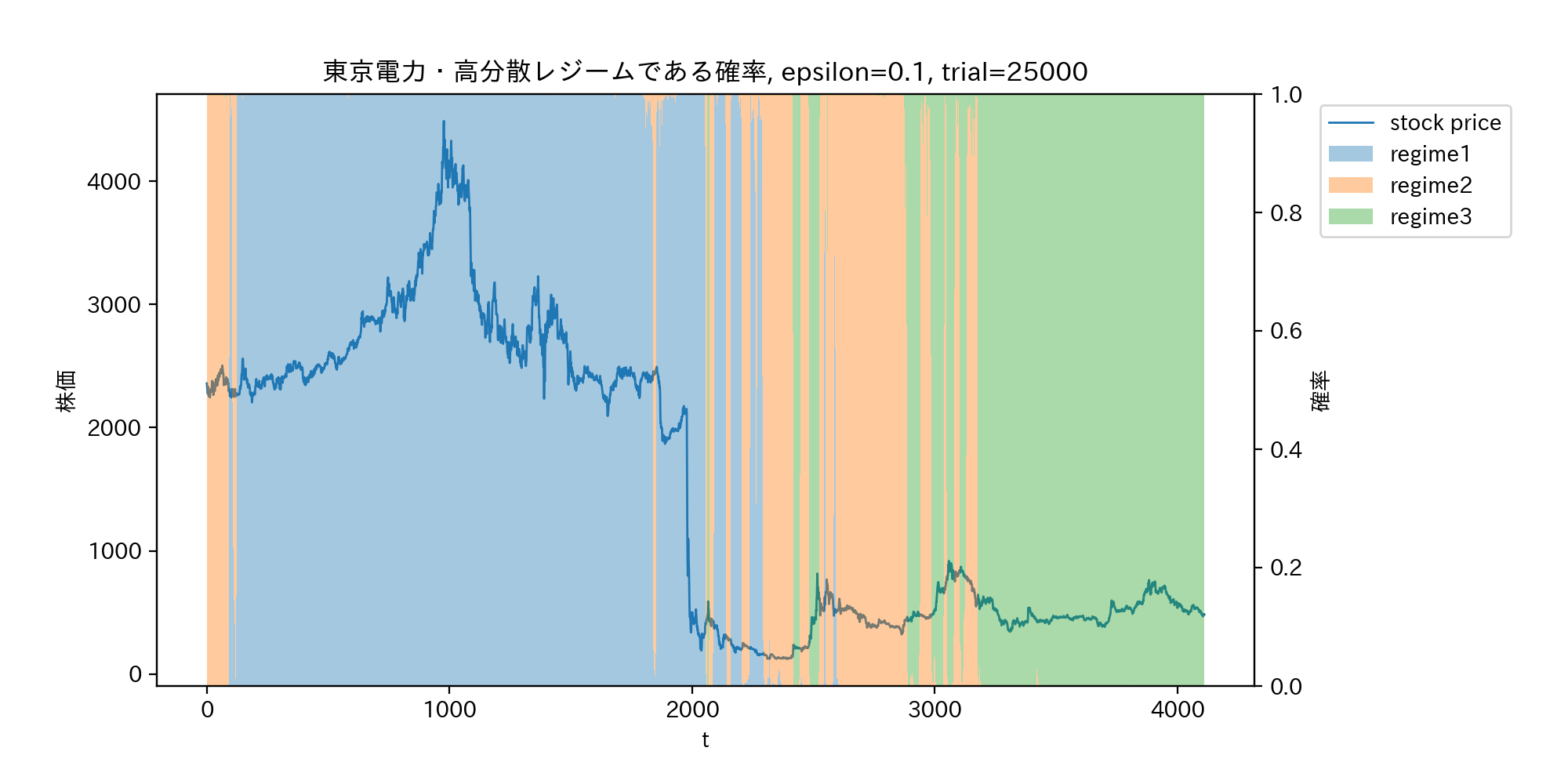
以下のグラフにおいて、高分散低収益率レジームを青、低分散低収益率レジームを黄色、中分散高収益レジームを緑とした。
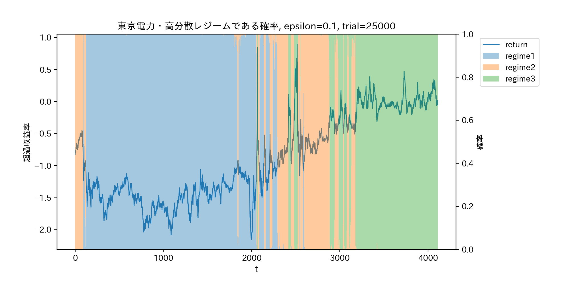
収益率ではなく、実際の株価をプロットしたのが下のグラフである。東日本大震災後の原発事故による株価の暴落は、レジームのスイッチではなくジャンプと推測されていることが分かる。
参考文献
- 小松高広(2018), 最適投資戦略 : ポートフォリオ・テクノロジーの理論と実践, 東京 : 朝倉書店
- 沖本竜義(2014), マルコフスイッチングモデルのマクロ経済・ファイナンスへの応用, 日本統計学会誌, 44 (1), 137-157