背景
- モデルを作成する際、事前に説明変数の分布を可視化したい
- 分布の可視化方法ついて、あまり記事を見かけないので私の実施している方法をまとめる。
対象データ
| 目的変数 | 説明変数 |
|---|---|
| 2値 | カテゴリ変数 |
サンプルデータ
MASSからデータ取得取得「低体重出生とそのリスク因子の関連」
library(MASS)

df <- birthwt
df <- within(df, {
  low <- factor(low, labels=c("No", "Yes"))
  lwt <- lwt * 0.454
  race <- factor(race, labels=c("White","Black","Other"))
  smoke <- factor(smoke, labels=c("No","Yes"))
  ptl <- factor(ptl)
  ht <- factor(ht, labels=c("No","Yes"))
  ui <- factor(ui, labels=c("No","Yes"))
  ftv <- factor(ftv)
})

df <- df[,c("low", "race", "ftv", "ptl")]
データ確認
head(df)
| low | race | ftv | ptl |
|---|---|---|---|
| No | Black | 0 | 0 |
| No | Other | 3 | 0 |
| No | White | 1 | 0 |
| No | White | 2 | 0 |
| No | White | 0 | 0 |
| No | Other | 0 | 0 |
やりたいこと
- カテゴリごとの件数
- カテゴリごとの目的変数(0,1)の割合
- 全体の目的変数(0,1)の割合
依存ライブラリ
library(dplyr)
library(ggplot2)
library(gtable)
library(gridExtra)
関数
binary_classification_plot_factor <- function(label, future, name){
  # make df
  df_marge <- data.frame(
    label=
      if(is.factor(label)){
        ifelse(as.integer(label)==2,1,0)
      }else{as.integer(label)}
    ,future=
      as.character(future)
    ,stringsAsFactors=FALSE)

  # make summary
  df_summary <-
    df_marge %>%
    group_by(future) %>%
    summarise(count=n(),avg_label=mean(label), sum_label=sum(label)) %>%
    as.data.frame

  # label sort
  df_summary$future <- factor(df_summary$future,levels=levels(future))

  # avg
  all_avg <- sum(df_summary$sum_label)/sum(df_summary$count)

  # plot
  p1 <- ggplot(data=df_summary)
  p1 <- p1 + geom_bar(aes(x=factor(future), y=count) ,stat="identity",fill="#515356",alpha=0.8)
  p1 <- p1 + theme_light() + xlab("category") + ylab("count(bar)") + labs(title=name)
  p1 <- p1 + theme(axis.text.x = element_text(angle=90, hjust = 1, vjust = 0.5))

  p2 <- ggplot(data=df_summary)
  p2 <- p2 + geom_point(aes(x=factor(future), y=avg_label), colour="#be0039", size=5)
  p2 <- p2 + geom_hline(yintercept=all_avg, color="#be0039", linetype="dashed")
  p2 <- p2 + xlab("category") + labs(title=name)
  p2 <- p2 + theme_light() %+replace%
    theme(panel.background = element_rect(fill = NA))

  g1 <- ggplot_gtable(ggplot_build(p1))
  g2 <- ggplot_gtable(ggplot_build(p2))

  pp <- c(subset(g1$layout, name == "panel", se = t:r))
  g <- gtable_add_grob(g1, g2$grobs[[which(g2$layout$name == "panel")]], pp$t,
                       pp$l, pp$b, pp$l)

  ia <- which(g2$layout$name == "axis-l")
  ga <- g2$grobs[[ia]]
  ax <- ga$children[[2]]
  ax$widths <- rev(ax$widths)
  ax$grobs <- rev(ax$grobs)
  ax$grobs[[1]]$x <- ax$grobs[[1]]$x - unit(1, "npc") + unit(0.15, "cm")
  g <- gtable_add_cols(g, g2$widths[g2$layout[ia, ]$l], length(g$widths) - 1)
  g <- gtable_add_grob(g, ax, pp$t, length(g$widths) - 1, pp$b)

  grid.arrange(g ,right = "category-rate(point), all-rate(line)")
}
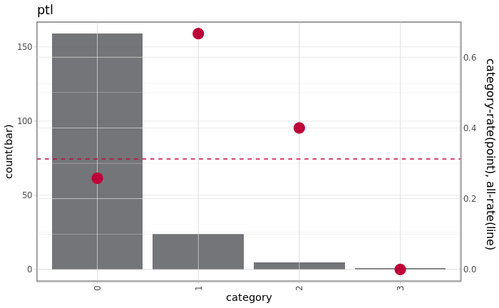
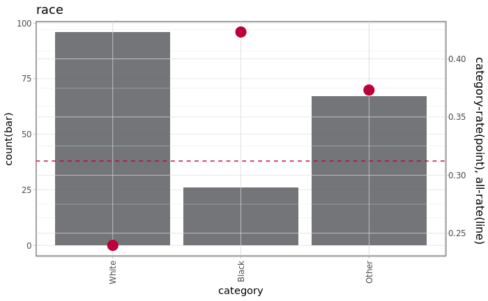
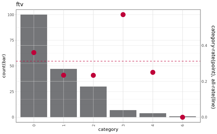
出力サンプル
binary_classification_plot_factor(df[,"low"], df[,"race"], "race")
binary_classification_plot_factor(df[,"low"], df[,"ftv"], "ftv")
binary_classification_plot_factor(df[,"low"], df[,"ptl"], "ptl")