GeForce GTX 1070 (8GB)
ASRock Z170M Pro4S [Intel Z170chipset]
Ubuntu 14.04 LTS desktop amd64
TensorFlow v0.11
cuDNN v5.1 for Linux
CUDA v8.0
Python 2.7.6
IPython 5.1.0 -- An enhanced Interactive Python.
gcc (Ubuntu 4.8.4-2ubuntu1~14.04.3) 4.8.4
GNU bash, version 4.3.8(1)-release (x86_64-pc-linux-gnu)
This article is related to ADDA (light scattering simulator based on the discrete dipole approximation).
In this article, pvec[] (polarization of dipoles) is displayed in 2D.
Note: (Apr. 17, 2017)
In this article, the pvec[] is displayed. However it is not actually the polarization of dipoles but axuiliary vectors used in the iterations.
So, the code in this article is NOT useful for people who want to display polarization of dipoles.
Reference: https://groups.google.com/forum/#!topic/adda-discuss/f3_Cm3HFtkA
Required
- UtilReadCoordinate.py
- UtilReadCheckPoint.py
- Coordinate file: coord.0
- produced with modified
iterative.c
- produced with modified
coord.0 was produced with the following:
$ ./adda -grid 25 -chp_type normal -chpoint 1s > log
v0.3
code
Jupyter code
from mpl_toolkits.mplot3d import Axes3D
import matplotlib.pyplot as plt
import matplotlib.cm as cm
import numpy as np
import sys
from UtilReadCoordinate import read_coordinate_file
from UtilReadCheckPoint import read_chpoint_file
'''
v0.3 Apr. 15, 2017
- display pvec[::3] in 2D
v0.2 Apr. 14, 2017
- use [sys.float_info.epsilon] for float comparison
v0.1 Apr. 10, 2017
- read checkpoint file
- read coordinate file
'''
res = read_coordinate_file('coord.0')
local_nvoid_Ndip, coord = res
res = read_chpoint_file('chp.0', 'aux.0')
itrgrp, auxgrp, vecgrp = res
print(local_nvoid_Ndip)
print(len(vecgrp.pvec))
xs, ys, zs = coord[::3], coord[1::3], coord[2::3]
pvc1, pvc2, pvc3 = vecgrp.pvec[::3], vecgrp.pvec[1::3], vecgrp.pvec[2::3]
plt_y1 = np.array([])
PICK_UP_ZZ_VALUE = -0.20943951023931953
SIZE_MAP_X, SIZE_MAP_Y = 50, 50
MIN_X, MIN_Y = -6, -6 # -6: based on coordinate values
RANGE_X = 6 - MIN_X # 6: based on coordinate values
RANGE_Y = 6 - MIN_Y # 6: based on coordinate values
rmap = [[0.0 for yi in range(SIZE_MAP_Y)] for xi in range(SIZE_MAP_X)]
for idx, xyz in enumerate(zip(xs, ys, zs)):
xx, yy, zz = xyz
if abs(zz - PICK_UP_ZZ_VALUE) >= sys.float_info.epsilon:
continue
xidx = int(SIZE_MAP_X * (xx - MIN_X) / RANGE_X )
yidx = int(SIZE_MAP_Y * (yy - MIN_Y) / RANGE_Y )
rmap[xidx][yidx] = pvc1[idx][0]
wrkarr = np.array(rmap)
figmap = np.reshape(wrkarr, (SIZE_MAP_X, SIZE_MAP_Y))
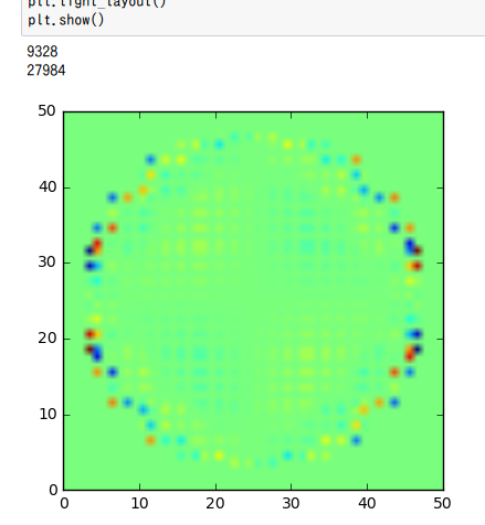
plt.imshow(figmap, extent=(0, SIZE_MAP_X, 0, SIZE_MAP_Y), cmap=cm.jet)
plt.tight_layout()
plt.show()
Re(pvec[::3])
Real part of the pvec[::3]
v0.6
Real and Imaginary part of dipoles (pvec) are displayed in 2D for quasi-median value of zs.
Those for electric field (xvec) are also diplayed.
code
Jupyter code.
from mpl_toolkits.mplot3d import Axes3D
import matplotlib.pyplot as plt
import matplotlib.cm as cm
import numpy as np
import sys

from UtilReadCoordinate import read_coordinate_file
from UtilReadCheckPoint import read_chpoint_file

'''
v0.6 Apr. 15, 2017
   - add show_xvec()
   - add show_pvec()
   - automatically calculate [PICK_UP_ZZ_VALUE]
v0.5 Apr. 15, 2017
   - change SIZE_MAP_X, SIZE_MAP_Y from [50, 50] to [30, 30]
   - use max() for RANG_X, RANGE_Y
   - use min() for MIN_X, MIN_Y
v0.4 Apr. 15, 2017
   - add add_figure()
v0.3 Apr. 15, 2017
   - display pvec[::3] in 2D
v0.2 Apr. 14, 2017
   - use [sys.float_info.epsilon] for float comparison
v0.1 Apr. 10, 2017
   - read checkpoint file
   - read coordinate file
'''

# codingrule: PEP8

res = read_coordinate_file('coord.0')
local_nvoid_Ndip, coord = res
res = read_chpoint_file('chp.0', 'aux.0')
itrgrp, auxgrp, vecgrp = res

print(local_nvoid_Ndip)
print(len(vecgrp.pvec))

xs, ys, zs = coord[::3], coord[1::3], coord[2::3]
pvc1, pvc2, pvc3 = vecgrp.pvec[::3], vecgrp.pvec[1::3], vecgrp.pvec[2::3]
xvc1, xvc2, xvc3 = vecgrp.xvec[::3], vecgrp.xvec[1::3], vecgrp.xvec[2::3]

plt_y1 = np.array([])
MARGIN_MINMAX = 1.0
#PICK_UP_ZZ_VALUE = -0.20943951023931953
wrk = np.unique(zs)
wrk = np.delete(zs, max(zs))
PICK_UP_ZZ_VALUE = np.median(wrk)
print('for Z=%f' % PICK_UP_ZZ_VALUE)


def add_figure(pick_up_zz, isRealPart, srcvec, dstplt):
    SIZE_MAP_X, SIZE_MAP_Y = 30, 30
    MIN_X, MIN_Y = min(xs) - MARGIN_MINMAX, min(ys) - MARGIN_MINMAX
    RANGE_X = max(xs) + MARGIN_MINMAX - MIN_X
    RANGE_Y = max(ys) + MARGIN_MINMAX - MIN_Y
    rmap = [[0.0 for yi in range(SIZE_MAP_Y)] for xi in range(SIZE_MAP_X)]

    for idx, xyz in enumerate(zip(xs, ys, zs)):
        xx, yy, zz = xyz
        if abs(zz - PICK_UP_ZZ_VALUE) >= sys.float_info.epsilon:
            continue
        xidx = int(SIZE_MAP_X * (xx - MIN_X) / RANGE_X)
        yidx = int(SIZE_MAP_Y * (yy - MIN_Y) / RANGE_Y)
        if isRealPart:
            rmap[xidx][yidx] = srcvec[idx][0]
        else:
            rmap[xidx][yidx] = srcvec[idx][1]

    wrkarr = np.array(rmap)
    figmap = np.reshape(wrkarr, (SIZE_MAP_X, SIZE_MAP_Y))
    dstplt.imshow(figmap, extent=(0, SIZE_MAP_X, 0, SIZE_MAP_Y), cmap=cm.jet)


def show_pvec():
    # 1. Real part of pvec[]
    plt.subplot(231)
    plt.title("Re{pvec}")
    add_figure(PICK_UP_ZZ_VALUE, True, pvc1, plt)
    plt.subplot(232)
    add_figure(PICK_UP_ZZ_VALUE, True, pvc2, plt)
    plt.subplot(233)
    add_figure(PICK_UP_ZZ_VALUE, True, pvc3, plt)
    # 2. Imaginary part of pvec[]
    plt.subplot(234)
    plt.title("Im{pvec}")
    add_figure(PICK_UP_ZZ_VALUE, False, pvc1, plt)
    plt.subplot(235)
    add_figure(PICK_UP_ZZ_VALUE, False, pvc2, plt)
    plt.subplot(236)
    add_figure(PICK_UP_ZZ_VALUE, False, pvc3, plt)

    plt.tight_layout()
    plt.show()


def show_xvec():
    # 1. Real part of pvec[]
    plt.subplot(231)
    plt.title("Re{xvec}")
    add_figure(PICK_UP_ZZ_VALUE, True, xvc1, plt)
    plt.subplot(232)
    add_figure(PICK_UP_ZZ_VALUE, True, xvc2, plt)
    plt.subplot(233)
    add_figure(PICK_UP_ZZ_VALUE, True, xvc3, plt)
    # 2. Imaginary part of pvec[]
    plt.subplot(234)
    plt.title("Im{xvec}")
    add_figure(PICK_UP_ZZ_VALUE, False, xvc1, plt)
    plt.subplot(235)

    add_figure(PICK_UP_ZZ_VALUE, False, xvc2, plt)
    plt.subplot(236)
    add_figure(PICK_UP_ZZ_VALUE, False, xvc3, plt)

    plt.tight_layout()
    plt.show()

show_pvec()
show_xvec()
Result
pvec[] : polarization of dipoles
xvec[] : total electric field on the dipoles
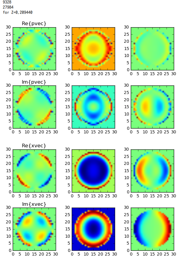
Fig2. From left to right: array[::3], array[1::3], arr[2::3].