GeForce GTX 1070 (8GB)
ASRock Z170M Pro4S [Intel Z170chipset]
Ubuntu 16.04 LTS desktop amd64
TensorFlow v1.2.1
cuDNN v5.1 for Linux
CUDA v8.0
Python 3.5.2
IPython 6.0.0 -- An enhanced Interactive Python.
gcc (Ubuntu 5.4.0-6ubuntu1~16.04.4) 5.4.0 20160609
GNU bash, version 4.3.48(1)-release (x86_64-pc-linux-gnu)
scipy v0.19.1
geopandas v0.3.0
MATLAB R2017b (Home Edition)
ADDA v.1.3b6
This article is related to ADDA (light scattering simulator based on the discrete dipole approximation).
Introduction
Light scattering properties of the nonspherical particles are studied for randomly orientated particles. For the random orientation averaging, there are two method:
- AOA (Analytical orientation averaging)
- NOA (Numerical orientation averaging)
Although the AOA is accurate, the method is limited for the shape of the particles (e.g. rotationally symmetric particles and particles such as Chebyshev particles). For the particles without the AOA, the NOA is used to obtain the light scattering properties.
The NOA is used with the configuration of the particle orientation based on the Euler angle ($\alpha$, $\beta$, and $\gamma$). Selection of the particle orientation sets have a influence on the computational efficiencies.
Hardin et al., 2016 studied the selection of popular point configuration on $S^2$. Those studied are as follows:
- Fibonacci and generalized spiral nodes
- projections of low discrepancy nodes from the unit square
- zonal equal area nodes and HEALPix nodes
- polygonal nodes such as icosahedral, cubed sphere, and octahedral nodes
- minimal energy nodes
- maximal determinant nodes
- random nodes
- mesh icosahedral equal area nodes
Hardin et al., 2016 shows properties of the above point configurations such as (1) equidistribution, (2) separation, (3) covering. The Mesh ratios are shown for each of the point configurations.
The point configurations shown in the paper can be obtained based on the MATLAB code by Grady Wright, which is available at spherepts @ GitHub. The code is partly exported to the Numpy and Scipy (for the Icosahedral nodes and Hammersley nodes: see. pySpherepts @ GitHub).
In this article, the priliminary results using the pySpherepts for the point sets are studied for the bisphere particles with the ADDA.
Particle configuration
The shape of the particle is the bisphere.
The properties of the bisphere are as follows:
- refractive index: m=1.5 + 0.005i
- equivolume sphere size parameter: 6.299605
- corresponds to
- radius of each composing sphere: 5.0
- equivolume sphere radius: 6.299605
- wavelength of the incident light: 2pi
- separation of the composing spheres
- touching (see below image)
-
-shape bisphere 1.0for ADDA
- box dimensions: 24x24x48
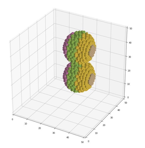
(Note: the color of the dipole shown above is only for the visualization, not for the different refractive indices)
NOA calculation (Random orientation averaging using [ADDA + pySpherepts])
Using the ADDA and pySpherepts, the random orientation averaging is performed for the Euler angle ($\beta$ and $\gamma$). In this study, the Euler angle $\alpha$ is fixeds as 0.0. The influence of the $\alpha$ is a future study.
The Qext (Extinction efficiency) is obtained using the code below together with the (ADDA + pySpherepts):
-
ADDA_pySpherepts_171217
- to obtain [beta_gamma.tbl]
-
loop_beta_gamma_171216.py
- to run sequentially ADDA for different values of [beta] and [gamma] for orientations by Euler angles ([alpha] is fixed as 0.0)
-
average_Qxxx_171216.py
- to average for Qext and Qabs for various values of the ADDA parameters
AOA calculation (bisphere.f)
Result for the AOA is obtained using the code based on the T-matrix method. The code (bisphere.f) is obtained from the https://www.giss.nasa.gov/staff/mmishchenko/t_matrix.html
Superposition T-matrix codes
Double-precision superposition T-matrix code for randomly oriented two-sphere clusters with externally touching or separated components: bisphere.f
The bisphere.f outputs Cext not Qext, where the Cext is the extinction cross section.
The conversion from the Cext to the Qext is performed using the calc_qext_bisphere_180104.py v0.4
Orientations for Hammersley nodes and Icosahedral nodes
Orientations for the Hammersley nodes are obtained for the given number of orientations N.
On the other hand, the number of orientations for the Icosahedral nodes is determined by the selection of the type and k index. For the type=0, the number of orientations for k index is shown below:
| kidx | #ori |
|---|---|
| 0 | 12 |
| 1 | 42 |
| 2 | 162 |
| 3 | 642 |
| 4 | 2562 |
| 5 | 10242 |
In this study, the k indices up to 4 (N=2562) are used for the Icosahedral nodes.
For the Hammersly nodes, the N is arbitrary obtained for (30, 60, 100, 300, 500, 1000, 1500, and 2000).
Result
Qext are obtained for the following:
- ADDA + Hammersley nodes
- res.qext_HammersleyNode_180106.txt
- ADDA + Icosahedral nodes
- res.qext_IcosNode_180106.txt
- bisphere.f
- res.qext_TMT_180106.txt
30,4.2360390
60,4.1844048
100,4.1664466
300,4.1657429
500,4.1631458
1000,4.1625290
1500,4.1625646
2000,4.1621403
12,4.1636192
42,4.2459419
162,4.1741279
642,4.1646836
2562,4.1624733
1,4.1440896
10000,4.1440896
Above results are plotted using Jupuyter + Matplotlib:
%matplotlib inline

import numpy as np
import matplotlib.pyplot as plt
from pylab import rcParams
from scipy.interpolate import spline

'''
v0.6 Jan. 06, 2018 comparison for [bisphere]
  - read results from T-matrix method [bisphere.f]
    + AOA(Analytical orientation averaging)
  - read results from [loop_HammersleyNode_180106_exec]
    + text manually extracted from the bash script result
v0.5 Dec. 24, 2017
  - add result for [avg_params.dat]
v0.4 Dec. 23, 2017
  - add result for [Icosahedral Nodes(type0)]
v0.3 Dec. 23, 2017
  - use original data for the .plot instead of interpolated one
v0.2 Dec. 23, 2017
  - fix bug: interpolated [out2] was 0.0
v0.1 Dec. 23, 2017
  - add lineplot
  - plot Qext as a scatterplot
'''

# rcParams['figure.figsize'] = 10,10
rcParams['figure.dpi'] = 130

# data1 = np.genfromtxt('res.qext_171217.txt', delimiter=',')
data1 = np.genfromtxt('res.qext_HammersleyNode_180106.txt', delimiter=',')
inp1 = np.array(data1[:,0])
out1 = np.array(data1[:,1])
# data2 = np.genfromtxt('res.qext_IcosNodes_171223.txt', delimiter=',')
data2 = np.genfromtxt('res.qext_IcosNode_180106.txt', delimiter=',')
inp2 = np.array(data2[:,0])
out2 = np.array(data2[:,1])
data3 = np.genfromtxt('res.qext_TMT_180106.txt', delimiter=',')
inp3 = np.array(data3[:,0])
out3 = np.array(data3[:,1])

fig = plt.figure()

ax1 = fig.add_subplot(1,1,1)

# 1. scatterplot
ax1.scatter(inp1, out1, label='ADDA + Hammersley nodes:NOA', color='blue', marker='o')
ax1.scatter(inp2, out2, label='ADDA + Icosahedral nodes(type0):NOA', color='red', marker='x')
ax1.scatter(inp3, out3, label='T-matrix(bisphere.f):AOA', color='green', marker='+')

# 2. lineplot
ax1.plot(inp1, out1, color='blue',  linestyle='solid')
ax1.plot(inp2, out2, color='red',  linestyle='solid')
ax1.plot(inp3, out3, color='green',  linestyle='solid')

ax1.set_title('-shape bisphere 1.0 -m 1.5 0.005 -eq_rad 6.299605')
ax1.set_xscale("log")
ax1.set_xlabel('# orientation')
ax1.set_ylabel('Qext')
ax1.grid(True)
ax1.legend()
ax1.set_xlim([1.0,10000.0])
ax1.set_ylim([3.8, 4.8])

# fig.show()

Errors and notes on the calculation
| A: NOA Qext | B: AOA Qext | abs(A-B) / B | |
|---|---|---|---|
| Hammersley nodes | 4.1621403 | 4.1440896 | 0.0043557 |
| Icosahedral nodes | 4.1624733 | 4.1440896 | 0.0044361 |
where N=2000 for Hammersley nodes and number of orientations is 2562 (k index=4) for Icosahedral nodes).
It is noted that the results for the NOA is obtained for fixed Euler angle $\alpha$(=0.0). Influence of the $\alpha$ has not been taken into account yet.
Result for Chebyshev particle

| A: NOA Qext | B: AOA Qext | abs(A-B) / B | |
|---|---|---|---|
| Hammersley nodes | 4.5204294 | ||
| Icosahedral nodes | 4.5204518 |
where N=2000 for Hammersley nodes and number of orientations is 2562 (k index=4) for Icosahedral nodes).
It is noted that the results for the NOA is obtained for fixed Euler angle $\alpha$(=0.0). Influence of the $\alpha$ has not been taken into account yet.