Quantopianについて
Quantopianは、Pythonを使って自動取引アルゴリズムをウェブ上で開発できます。
Quantopianでは、バックテストやポートフォリオ分析の仕組みをオープンソース化しており、バックテスト等の膨大なデータを扱う処理もクラウド上で完結している、完全無料のサービスです。
また、Quantpianには多数のAPIが存在しており、リサーチ環境でアルゴリズムに活用するデータを参照することが可能となっております。
Quantopianの始め方
アカウント登録が完了したら、以下チュートリアルのぺーじに沿って進めると良いでしょう。
https://www.quantopian.com/get-funded
Researchを活用する
データの探索1
QuantopianのResearch機能は、アメリカの8,000以上ある株式の2002年以降の、価格やボリューム、リターンなどを自由に取り扱うことができます。
早速ですが、Appleの株価データを調査してみましょう。
# Research environment functions
from quantopian.research import prices, symbols

# Pandas library: https://pandas.pydata.org/
import pandas as pd

# Query historical pricing data for AAPL
aapl_close = prices(
    assets=symbols('AAPL'),
    start='2013-01-01',
    end='2016-01-01',
)

# Compute 20 and 50 day moving averages on
# AAPL's pricing data
aapl_sma20 = aapl_close.rolling(20).mean()
aapl_sma50 = aapl_close.rolling(50).mean()

# Combine results into a pandas DataFrame and plot
pd.DataFrame({
    'AAPL': aapl_close,
    'SMA20': aapl_sma20,
    'SMA50': aapl_sma50
}).plot(
    title='AAPL Close Price / SMA Crossover'
);
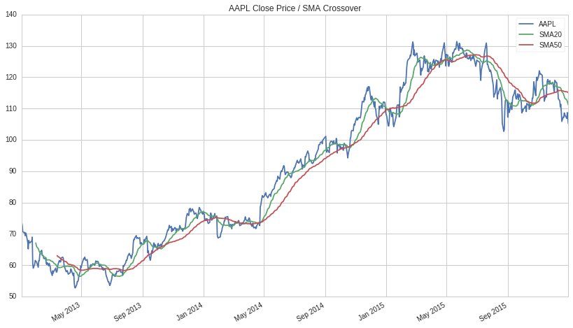
こちらのコードを実行すると、以下のようなAppleの株価/移動平均線20/移動平均線50のグラフが描けると思います。
Pipeline API
PipelineのAPIは横断的な分析に対して非常に有効です。複数のインプットされたデータを集計したり、時系列データの分析を行ったりすることが可能です。
APIを活用し、以下3つのようなことが可能です。
・フィルタリングルールに基づく株式の選定
・スコアリング関数に基づく株式のランク付け
・最適なポートフォリオの計算
それでは、さっそくパイプラインをインポートしてみましょう。
# Pipeline class
from quantopian.pipeline import Pipeline

def make_pipeline():
    # Create and return an empty Pipeline
    return Pipeline()
アウトプットをパイプラインに追加するため、データセットを参照し、実行したいデータを特定する必要があります。例えば、close のcolumnを利用する場合、 USEquityPricing のデータセットを参照します。そして、以下のように最新の株価をこのカラムから定義することが可能となっています。
# Import Pipeline class and USEquityPricing dataset
from quantopian.pipeline import Pipeline
from quantopian.pipeline.data import USEquityPricing

def make_pipeline():
    # Get latest closing price
    close_price = USEquityPricing.close.latest

    # Return Pipeline containing latest closing price
    return Pipeline(
        columns={
            'close_price': close_price,
        }
    )
Pipeline APIには、いくつかの組み込み計算も用意されています。例えば次のコードは Psychsignal の stocktwits データセットをインポートし、出力をその bull_minus_bear 列の3日間の移動平均として定義します。
# Import Pipeline class and datasets
from quantopian.pipeline import Pipeline
from quantopian.pipeline.data import USEquityPricing
from quantopian.pipeline.data.psychsignal import stocktwits

# Import built-in moving average calculation
from quantopian.pipeline.factors import SimpleMovingAverage


def make_pipeline():
    # Get latest closing price
    close_price = USEquityPricing.close.latest

    # Calculate 3 day average of bull_minus_bear scores
    sentiment_score = SimpleMovingAverage(
        inputs=[stocktwits.bull_minus_bear],
        window_length=3,
    )

    # Return Pipeline containing close_price
    # and sentiment_score
    return Pipeline(
        columns={
            'close_price': close_price,
            'sentiment_score': sentiment_score,
        }
    )
戦略を構築する上で大切なことは、ポートフォリオに組み込む株式を設定することです。一方でQuantopianではできる限り流動性の高い株式が適切だと考えています。
Quantopianの QTradableStocksUS はこの特徴付を行っています。
# Import Pipeline class and datasets
from quantopian.pipeline import Pipeline
from quantopian.pipeline.data import USEquityPricing
from quantopian.pipeline.data.psychsignal import stocktwits

# Import built-in moving average calculation
from quantopian.pipeline.factors import SimpleMovingAverage

# Import built-in trading universe
from quantopian.pipeline.experimental import QTradableStocksUS


def make_pipeline():
    # Create a reference to our trading universe
    base_universe = QTradableStocksUS()

    # Get latest closing price
    close_price = USEquityPricing.close.latest

    # Calculate 3 day average of bull_minus_bear scores
    sentiment_score = SimpleMovingAverage(
        inputs=[stocktwits.bull_minus_bear],
        window_length=3,
    )

    # Return Pipeline containing close_price and
    # sentiment_score that has our trading universe as screen
    return Pipeline(
        columns={
            'close_price': close_price,
            'sentiment_score': sentiment_score,
        },
        screen=base_universe,
    )
これでPipelineの定義は完全に完了し、run_pipeline を利用すれば特定の期間のデータを実行することができます。
アウトプットは日付と株ごとのpandasのDataFrameとなります。
# Import run_pipeline method
from quantopian.research import run_pipeline

# Execute pipeline created by make_pipeline
# between start_date and end_date
pipeline_output = run_pipeline(
    make_pipeline(),
    start_date='2013-01-01',
    end_date='2013-12-31'
)

# Display last 10 rows
pipeline_output.tail(10)
戦略の定義
ここまでのチュートリアルでどのようにデータにアクセスするかは理解頂けたと思います。
ここからは、ロング・ショート戦略を構築しましょう。
一般に、ロング・ショート戦略は、試算の相対的価値をモデル化を行い、値上がりが期待できる割安な銘柄(過小評価された銘柄)を買い、同時に値下がりが予想される割高な銘柄(過大評価された銘柄)を空売りします。
戦略 :過去3日間のセンチメントスコアが高いものは高い株価とみなし、低いものは低い株価とみなします。
戦略分析
先程行ったものと同様に、 SimpleMovingAverage と stocktwits と bull_minus_bearのデータを定義できます。
# Pipeline imports
from quantopian.pipeline import Pipeline
from quantopian.pipeline.data.psychsignal import stocktwits
from quantopian.pipeline.factors import SimpleMovingAverage
from quantopian.pipeline.experimental import QTradableStocksUS


# Pipeline definition
def  make_pipeline():

    base_universe = QTradableStocksUS()

    sentiment_score = SimpleMovingAverage(
        inputs=[stocktwits.bull_minus_bear],
        window_length=3,
    )

    return Pipeline(
        columns={
            'sentiment_score': sentiment_score,
        },
        screen=base_universe
    )
シンプルに、 sentiment_score トップ350と下位350のみを分析します。
top と bottom のメソッドくを活用することにより、パイプラインのフィルターを作成することが可能です。そして、フィルターと取引量の方針を通して他の余分な株価を取り除くことが可能です。
# Pipeline imports
from quantopian.pipeline import Pipeline
from quantopian.pipeline.data.psychsignal import stocktwits
from quantopian.pipeline.factors import SimpleMovingAverage
from quantopian.pipeline.experimental import QTradableStocksUS

# Pipeline definition
def  make_pipeline():

    base_universe = QTradableStocksUS()

    sentiment_score = SimpleMovingAverage(
        inputs=[stocktwits.bull_minus_bear],
        window_length=3,
    )

    # Create filter for top 350 and bottom 350
    # assets based on their sentiment scores
    top_bottom_scores = (
        sentiment_score.top(350) | sentiment_score.bottom(350)
    )

    return Pipeline(
        columns={
            'sentiment_score': sentiment_score,
        },
        # Set screen as the intersection between our filter
        # and trading universe
        screen=(
            base_universe
            & top_bottom_scores
        )
    )
次に、私達が分析を行いたい期間のデータを実行します。
ここでは2018/1/1~2018/12/31までのデータとしております。
# Import run_pipeline method
from quantopian.research import run_pipeline

# Specify a time range to evaluate
period_start = '2018-01-01'
period_end = '2018-12-31'

# Execute pipeline over evaluation period
pipeline_output = run_pipeline(
    make_pipeline(),
    start_date=period_start,
    end_date=period_end
)```


Pipelineのデータに加え、株価データが必要となりますので。これは容易に出力することが可能で、 `prices`を参照します。

```python
# Import prices function
from quantopian.research import prices

# Get list of unique assets from the pipeline output
asset_list = pipeline_output.index.levels[1].unique()

# Query pricing data for all assets present during
# evaluation period
asset_prices = prices(
    asset_list,
    start=period_start,
    end=period_end
)
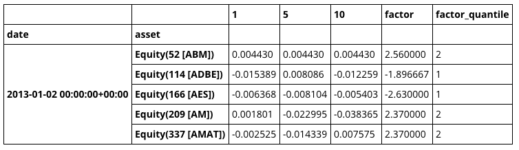
戦略をテストするために、Quantopianのオープンソースである Alphalens を活用することができます。最初に、get_clean_factor_and_forward_returns を利用し、 factor pricing のデータを結合しましょう。
# Import Alphalens
import alphalens as al

# Get asset forward returns and quantile classification
# based on sentiment scores
factor_data = al.utils.get_clean_factor_and_forward_returns(
    factor=pipeline_output['sentiment_score'],
    prices=asset_prices,
    quantiles=2,
    periods=(1,5,10),
)

# Display first 5 rows
factor_data.head(5)
このデータフォーマットを活用することにより、いくつかのAlphalensによる分析が行えます。
では、期間全体の平均リターンをみることから始めましょう。
あくまでも、目標はロング・ショート戦略を構築することです。
# Calculate mean return by factor quantile
mean_return_by_q, std_err_by_q = al.performance.mean_return_by_quantile(factor_data)
# Plot mean returns by quantile and holding period
# over evaluation time range
al.plotting.plot_quantile_returns_bar(
mean_return_by_q.apply(
al.utils.rate_of_return,
axis=0,
args=('1D',)
)
);```

また、次のコードを利用して、保有期間5日間ののロング・ショートポートフォリオの累積リターンをプロットすることができます。
```python
# Calculate factor-weighted long-short portfolio returns
ls_factor_returns = al.performance.factor_returns(factor_data)
# Plot cumulative returns for 5 day holding period
al.plotting.plot_cumulative_returns(ls_factor_returns['5D'], '5D');
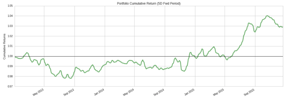
上のプロットは大きなドローダウン期間を示しており、この分析ではまだ取引コストや市場への影響を考慮していません。 ここから、Alphalensを活用し、より深い分析を行い、戦略のアイデアを繰り返すべきです。
Algorithm API & Core Functions
ここからは、QuantopianのアルゴリズムAPIを活用し、基本的なトレード戦略を構築していきます。
アルゴリズムAPIは注文の決定とスケジューリング、そしてアルゴリズムのパラメーターの初期化と管理を行います。
それでは、いくつか核となる関数をみていきましょう。
initialize(context)
initialize はアルゴリズムをスタートする1回と、 context を必要とする時のみ利用します。
context は、シミュレーションプロセス全体を通して状態を維持するために使用されるPython辞書であり、アルゴリズムのさまざまな部分で参照できます。
関数を呼び出す際に、永続化したい変数は、グローバル変数を使用するのではなく、 context に格納する必要があります。ドット記法(context.some_attribute)を使用して、コンテキスト変数にアクセスして初期化することができます。
before_trading_start(context, data)
before_trading_start は、マーケットがオープンする前に1日1回呼び出され、入力としてcontextとデータを必要とします。 context は initialize からの同じ辞書への参照です。 data は、任意のアセットの現在または過去の価格設定と、ボリュームを調べることを可能にするいくつかのAPI関数を格納するオブジェクトです。
before_trading_start は、パイプラインの出力を取得する場所でもあります。また、ポートフォリオ構築に使用する前に、結果データの前処理を行います。 これについては次のチュートリアルで説明します。
schedule_function(func, day_rule, time_rule)
Quantopianでは、アルゴリズムはNYSEの取引カレンダーに従って、通常の取引日の午前9時30分から午後4時の間に株式を取引できます。
schedule_function を使用すると、指定した日時にカスタム関数を実行できます。
たとえば、次のように、各週の初日にマーケットオープンでポートフォリオをリバランスする機能をスケジュールできます。
schedule_function(
    rebalance,
    date_rule=date_rules.week_start(),
    time_rule=time_rules.market_open()
)
スケジューリング関数は初期化時に実行する必要があり、このメソッドでスケジューリングされたカスタム関数は引数として、context と data を受け取る必要があります。 利用可能な date_rules と time_rules の完全なリストは、 Quantopianのドキュメント をチェックしてください。
次に、取引アルゴリズムの骨格を作りましょう。 現状、アルゴリズムはシミュレーションで経過した日数を追跡し、日付と時刻に応じて異なるメッセージを記録します。
# Import Algorithm API
import quantopian.algorithm as algo


def initialize(context):
    # Initialize algorithm parameters
    context.day_count = 0
    context.daily_message = "Day {}."
    context.weekly_message = "Time to place some trades!"

    # Schedule rebalance function
    algo.schedule_function(
        rebalance,
        date_rule=algo.date_rules.week_start(),
        time_rule=algo.time_rules.market_open()
    )


def before_trading_start(context, data):
    # Execute any daily actions that need to happen
    # before the start of a trading session
    context.day_count += 1
    log.info(context.daily_message, context.day_count)


def rebalance(context, data):
    # Execute rebalance logic
    log.info(context.weekly_message)
ここまでで、取引あるごリズムのための基本的な構造ができました。
アルゴリズムにおけるデータ処理
次に、Research で構築したデータパイプラインにアルゴリズムに統合します。
Research との重要な違いの1つは、バックテスト中にシミュレーションが進行するにつれてパイプラインが毎日実行されるため、 start_date と end_date 引数を含める必要がないことです。
アルゴリズムでデータパイプラインを使用するための最初のステップは、アルゴリズムの初期化関数にそれへの参照を追加することです。 これは、2つの入力を必要とする attach_pipeline メソッドを使用して行われます。
これは、 make_pipeline を使用して構築する Pipeline オブジェクトへの参照と、それを識別するためのString名です。
# Import Algorithm API
import quantopian.algorithm as algo


def initialize(context):
    # Attach pipeline to algorithm
    algo.attach_pipeline(
        make_pipeline(),
        'data_pipe'
    )

    # Schedule rebalance function
    algo.schedule_function(
        rebalance,
        date_rule=algo.date_rules.week_start(),
        time_rule=algo.time_rules.market_open()
    )


def before_trading_start(context, data):
    pass


def rebalance(context, data):
    pass
上記のように、Quantopianのパイプラインは、毎日市場が開かれる前にデータストリームを処理して出力を生成します。
初期化で指定したパイプライン名を取り、パイプラインによって生成されたPandasのDataFrameを返す、 pipeline_output関数を使用して、 before_trading_start でパイプラインの出力を取得できます。
今のところ、リバランス機能を使用して、パイプラインの出力から上位10行をログに記録できます。
# Import Algorithm API
import quantopian.algorithm as algo


def initialize(context):
    # Attach pipeline to algorithm
    algo.attach_pipeline(
        make_pipeline(),
        'data_pipe'
    )

    # Schedule rebalance function
    algo.schedule_function(
        rebalance,
        date_rule=algo.date_rules.week_start(),
        time_rule=algo.time_rules.market_open()
    )


def before_trading_start(context, data):
    # Get pipeline output and
    # store it in context
    context.pipeline_data = algo.pipeline_output(
        'data_pipe'
    )


def rebalance(context, data):
    # Display first 10 rows
    # of pipeline output
    log.info(context.pipeline_data.head(10))
次に、 Research で構築した make_pipeline 関数をアルゴリズムに追加しましょう。
分析のために行ったように資産の数を制限するのではなく、アルゴリズムはそれがセンチメントスコアを持っている取引すべての資産を考慮するべきです。
これには、 sentiment_score 出力の notnull メソッドを使用してフィルタを作成し、 &演算子 を使用して取引可能なユニバースとの共通部分を取得します。
# Import Algorithm API
import quantopian.algorithm as algo

# Pipeline imports
from quantopian.pipeline import Pipeline
from quantopian.pipeline.data.psychsignal import stocktwits
from quantopian.pipeline.factors import SimpleMovingAverage
from quantopian.pipeline.filters import QTradableStocksUS


def initialize(context):
    # Attach pipeline to algorithm
    algo.attach_pipeline(
        make_pipeline(),
        'data_pipe'
    )

    # Schedule rebalance function
    algo.schedule_function(
        rebalance,
        date_rule=algo.date_rules.week_start(),
        time_rule=algo.time_rules.market_open()
    )


def before_trading_start(context, data):
    # Get pipeline output and
    # store it in context
    context.pipeline_data = algo.pipeline_output('data_pipe')


def rebalance(context, data):
    # Display first 10 rows
    # of pipeline output
    log.info(context.pipeline_data.head(10))


# Pipeline definition
def make_pipeline():

    base_universe = QTradableStocksUS()

    sentiment_score = SimpleMovingAverage(
        inputs=[stocktwits.bull_minus_bear],
        window_length=3,
    )

    return Pipeline(
        columns={
            'sentiment_score': sentiment_score,
        },
        screen=(
            base_universe
            & sentiment_score.notnull()
        )
    )
これで、取引可能な資産の範囲を毎日選択し、ポートフォリオ内の資産配分を決定するために使用できるアルファスコアを生成ができました。
Portfolio Management
ここでは、パイプラインで生成されたアルファスコアをアルゴリズムがどのように使用してポートフォリオのバランスを取り戻すかを定義します。 目標は、一連のルールや制約によって定義された特定の構造を維持しながら、アルファスコアに基づいて収益を最大化するターゲットポートフォリオを見つけることです。
これは、ポートフォリオ最適化問題と呼ばれます。 QuantopianのOptimize APIを使用すると、パイプラインの出力を目的と一連の制約に簡単に変換できます。
その後、 order_optimal_portfolio を使用して、現在のポートフォリオを、仕様を満たすターゲットポートフォリオに移行できます。 最初のステップは目的を定義することです。 MaximizeAlpha を使用します。これは、アルファスコアに比例して資本を資産に割り当てようとします。
# Import Optimize API module
import quantopian.optimize as opt


def rebalance(context, data):
  # Retrieve alpha from pipeline output
  alpha = context.pipeline_data.sentiment_score

  if not alpha.empty:
      # Create MaximizeAlpha objective
      objective = opt.MaximizeAlpha(alpha)
次に、ターゲットポートフォリオに満たさせたい制約のリストを指定する必要があります。
初期化でいくつかのしきい値を定義し、それらを context 変数に格納することから始めましょう。
# Constraint parameters
context.max_leverage = 1.0
context.max_pos_size = 0.015
context.max_turnover = 0.95
これで、上で定義したしきい値を使用して、リバランスにおける制約を指定できます。
# Import Optimize API module
import quantopian.optimize as opt


def rebalance(context, data):
  # Retrieve alpha from pipeline output
  alpha = context.pipeline_data.sentiment_score

  if not alpha.empty:
      # Create MaximizeAlpha objective
      objective = opt.MaximizeAlpha(alpha)

      # Create position size constraint
      constrain_pos_size = opt.PositionConcentration.with_equal_bounds(
          -context.max_pos_size,
          context.max_pos_size
      )

      # Constrain target portfolio's leverage
      max_leverage = opt.MaxGrossExposure(context.max_leverage)

      # Ensure long and short books
      # are roughly the same size
      dollar_neutral = opt.DollarNeutral()

      # Constrain portfolio turnover
      max_turnover = opt.MaxTurnover(context.max_turnover)
最後に、目的のポートフォリオと制約のリストを order_optimal_portfolio に渡してターゲットポートフォリオを計算し、現在のポートフォリオを最適な状態に移行するのに必要な注文を発信できます。
# Import Algorithm API
import quantopian.algorithm as algo

# Import Optimize API
import quantopian.optimize as opt


def rebalance(context, data):
  # Retrieve alpha from pipeline output
  alpha = context.pipeline_data.sentiment_score

  if not alpha.empty:
      # Create MaximizeAlpha objective
      objective = opt.MaximizeAlpha(alpha)

      # Create position size constraint
      constrain_pos_size = opt.PositionConcentration.with_equal_bounds(
          -context.max_pos_size,
          context.max_pos_size
      )

      # Constrain target portfolio's leverage
      max_leverage = opt.MaxGrossExposure(context.max_leverage)

      # Ensure long and short books
      # are roughly the same size
      dollar_neutral = opt.DollarNeutral()

      # Constrain portfolio turnover
      max_turnover = opt.MaxTurnover(context.max_turnover)

      # Rebalance portfolio using objective
      # and list of constraints
      algo.order_optimal_portfolio(
          objective=objective,
          constraints=[
              constrain_pos_size,
              max_leverage,
              dollar_neutral,
              max_turnover,
          ]
      )
リスク管理
目標ポートフォリオの構造に対する制約を設定することに加えて、その業績に影響を及ぼし得る共通のリスク要因に対するそのエクスポージャーを制限したいと思います。
例えば、株価指数のセンチメントデータは一時的なものであり、センチメントスコアの急上昇を利用するという意図のために、アルゴリズムは短期の逆転リスクにさらされる可能性があります。
ポートフォリオの共通リスク要因に対するエクスポージャーを管理するためにQuantopianのリスクモデルを使用します。
リスクモデルは、11のセクター要因と5つのスタイル要因(短期の組戻しを含む)の16種類のリスク要因に対する、資産エクスポージャーを計算します。 risk_loading_pipeline 関数を使用すると、リスクモデルの各因子について出力列を生成するデータパイプラインを返すので、アルゴリズム内でこのデータに簡単にアクセスできます。 データパイプラインと同様に、リスクデータパイプラインをアルゴリズムに付加し、それを識別するための名前を指定する必要があります。 それから、その出力を before_trading_start に入れて、コンテキストに格納することができます。
# Import Algorithm API
import quantopian.algorithm as algo

# Import Risk API method
from quantopian.pipeline.experimental import risk_loading_pipeline

def initialize(context):
    # Constraint parameters
    context.max_leverage = 1.0
    context.max_pos_size = 0.015
    context.max_turnover = 0.95

    # Attach data pipelines
    algo.attach_pipeline(
        make_pipeline(),
        'data_pipe'
    )
    algo.attach_pipeline(
        risk_loading_pipeline(),
        'risk_pipe'
    )

    # Schedule rebalance function
    algo.schedule_function(
        rebalance,
        algo.date_rules.week_start(),
        algo.time_rules.market_open(),
    )


def before_trading_start(context, data):
    # Get pipeline outputs and
    # store them in context
    context.pipeline_data = algo.pipeline_output(
      'data_pipe'
    )

    context.risk_factor_betas = algo.pipeline_output(
      'risk_pipe'
    )
次のステップは、 RiskModelExposure 制約をポートフォリオ最適化ロジックに追加することです。
この制約は、リスクモデルによって生成されたデータを使用して、モデルに含まれる各要因に対するターゲットポートフォリオの全体的なエクスポージャーに制限を設定します。
# Constrain target portfolio's risk exposure
# By default, max sector exposure is set at
# 0.2, and max style exposure is set at 0.4
factor_risk_constraints = opt.experimental.RiskModelExposure(
    context.risk_factor_betas,
    version=opt.Newest
)
最後に、以下のアルゴリズムは、戦略とポートフォリオ構築ロジックを網羅しており、バックテストの準備ができています。
# Import Algorithm API
import quantopian.algorithm as algo

# Import Optimize API
import quantopian.optimize as opt

# Pipeline imports
from quantopian.pipeline import Pipeline
from quantopian.pipeline.data.psychsignal import stocktwits
from quantopian.pipeline.factors import SimpleMovingAverage

# Import built-in universe and Risk API method
from quantopian.pipeline.filters import QTradableStocksUS
from quantopian.pipeline.experimental import risk_loading_pipeline


def initialize(context):
    # Constraint parameters
    context.max_leverage = 1.0
    context.max_pos_size = 0.015
    context.max_turnover = 0.95

    # Attach data pipelines
    algo.attach_pipeline(
        make_pipeline(),
        'data_pipe'
    )
    algo.attach_pipeline(
        risk_loading_pipeline(),
        'risk_pipe'
    )

    # Schedule rebalance function
    algo.schedule_function(
        rebalance,
        algo.date_rules.week_start(),
        algo.time_rules.market_open(),
    )


def before_trading_start(context, data):
    # Get pipeline outputs and
    # store them in context
    context.pipeline_data = algo.pipeline_output('data_pipe')

    context.risk_factor_betas = algo.pipeline_output('risk_pipe')


# Pipeline definition
def make_pipeline():

    sentiment_score = SimpleMovingAverage(
        inputs=[stocktwits.bull_minus_bear],
        window_length=3,
        mask=QTradableStocksUS()
    )

    return Pipeline(
        columns={
            'sentiment_score': sentiment_score,
        },
        screen=sentiment_score.notnull()
    )


def rebalance(context, data):
    # Retrieve alpha from pipeline output
    alpha = context.pipeline_data.sentiment_score

    if not alpha.empty:
        # Create MaximizeAlpha objective
        objective = opt.MaximizeAlpha(alpha)

        # Create position size constraint
        constrain_pos_size = opt.PositionConcentration.with_equal_bounds(
            -context.max_pos_size,
            context.max_pos_size
        )

        # Constrain target portfolio's leverage
        max_leverage = opt.MaxGrossExposure(context.max_leverage)

        # Ensure long and short books
        # are roughly the same size
        dollar_neutral = opt.DollarNeutral()

        # Constrain portfolio turnover
        max_turnover = opt.MaxTurnover(context.max_turnover)

        # Constrain target portfolio's risk exposure
        # By default, max sector exposure is set at
        # 0.2, and max style exposure is set at 0.4
        factor_risk_constraints = opt.experimental.RiskModelExposure(
            context.risk_factor_betas,
            version=opt.Newest
        )

        # Rebalance portfolio using objective
        # and list of constraints
        algo.order_optimal_portfolio(
            objective=objective,
            constraints=[
                constrain_pos_size,
                max_leverage,
                dollar_neutral,
                max_turnover,
                factor_risk_constraints,
            ]
        )
バックテストでの分析
バックテストが終了したら、[Notebook]タブをクリックしてください。

これにより、以下のコードを含む Research ノートブックが表示されます。
bt = get_backtest('5a4e4faec73c4e44f218170a')
bt.create_full_tear_sheet()
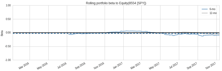
もう1つの興味深い部分は、パフォーマンス属性セクションです。
以下のプロットは、Quantopianのリスクモデルを使用して、収益のどれだけがあなたの戦略に起因しているのか、そしてそのどれだけが共通のリスク要因から生じているのかを示しています。
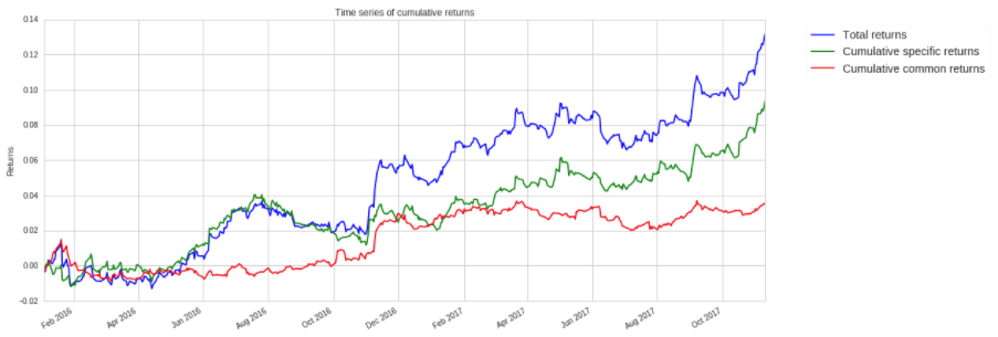
上記のように、ポートフォリオの総収益の大部分は特定の収益から生じています。
これは、アルゴリズムのパフォーマンスが一般的なリスク要因にさらされているためではないことを示しており、これは良いことです。
これで、チュートリアル1は終了となります。