この記事の続きはこちら
Rの練習として
R言語を学び始めた。
ごく基本的なことがわかったところで、ひとまずやってみようと思いついたのは、力学の多体問題を数値的に解くこと。
「データをベクトルで処理する」というRの仕組みが、多変数の連立微分方程式を解くのに向いているんじゃないかと思ったのだ。
Rの用途としてアリなのかどうかは微妙な気もするが、勉強のため、ということで。
これは何
$n$個 の質点が互いに力を及ぼしあい、また外力を受けて運動している系を考える。
これら $n$個 の質点のNewton力学による運動方程式を古典的Runge-Kutta法で解いて、結果を
- 画面に描く
- 時刻・質点の位置・質点の速度 のテキストファイルにする
- 画像ファイルにして保存する
というプログラム。
いろいろな問題を解けるように汎用性を重視して、Runge-Kuttaの計算を行うエンジン部分と運動方程式の右辺のベクトルを計算する関数とを分離した。
テストとして、単振り子、バネで連結した質点モデルによる1次元の波動の伝播、同じく2次元の波動の伝播の問題を解いてみたぞ。
いちおう、うまくいった(ように見える)。
環境
Ubuntu20.04
R3.6.3
Core i7-7700HQ 2.80GHzx8
メモリ16GB
理屈
運動方程式
簡単な場合として1次元を考えると
Newton力学の運動方程式は
$\displaystyle m \hspace{0.1em} \ddot{r} = f(t,r,v)$
( $t$ : 時刻 , $r$ : 座標 , $v$ : 速度 , $f(t,r,v)$ : $t$ と $r$ と $v$ の関数 )
これは2階の線形微分方程式。
Runge-Kutta法は1階の微分方程式を解くので、このままでは解けない。
こういうときは、次のようにすると、2階微分方程式を2次元の1階微分方程式に置き換えられる。
$r$ と $v$ の2つを独立変数とみなす。すると
$\dot{r} = v$
$\dot{v} = \mbox{運動方程式で与えられる}$
すなわち
$\dot{r} = v$
$\displaystyle \dot{v} = \frac{1}{m} \hspace{0.1em} f(t,r,v)$
と表せる。
要するに、 $( r , v )$ をまとめて $\mathbf r$ と書いて1つの変数(ベクトル)とみなせば
$\dot{\mathbf r} = f'(t,{\mathbf r})$
( $f'(t,{\mathbf r})$ : $t$ と $\mathbf r$ の関数)
という、1階の微分方程式として扱える。
これならRunge-Kutta法で解ける!
古典的Runge-Kutta法
ある 時刻 $t_{0}$ における質点の 位置と速度 $\mathbf r_{0}$ がわかっているとする。
運動方程式を表す 関数 $f'(t,{\mathbf r})$ が与えられているとする。
このとき、微小な 時間 ${\mit\Delta} t$ 後までの 位置と速度の変化 ${\mit\Delta}{\mathbf r}$ を、次の公式を使って、 ${\mit\Delta} t$ の4次の精度で求めることができる。
$\displaystyle t_{1} = t_{0} + \frac{{\mit\Delta} t}{2}$
$\displaystyle t_{2} = t_{0} + {\mit\Delta} t$
$\displaystyle {\mathbf r_{1}} = {\mathbf r_{0}} + {\mathbf k_{0}} \hspace{0.1em} \frac{{\mit\Delta} t}{2}$
$\displaystyle {\mathbf r_{2}} = {\mathbf r_{0}} + {\mathbf k_{1}} \hspace{0.1em} \frac{{\mit\Delta} t}{2}$
$\displaystyle {\mathbf r_{3}} = {\mathbf r_{0}} + {\mathbf k_{2}} \hspace{0.1em} {\mit\Delta} t$
${\mathbf k_{0}} = f'(t_{0},{\mathbf r_{0}})$
$\displaystyle {\mathbf k_{1}} = f' ( t_{1} , {\mathbf r_{1}} )$
$\displaystyle {\mathbf k_{2}} = f' ( t_{1} , {\mathbf r_{2}} )$
$\displaystyle {\mathbf k_{3}} = f' ( t_{2} , {\mathbf r_{3}} )$
$\displaystyle {\mit\Delta} {\mathbf r} = \frac{1}{6} \hspace{0.1em} ( \hspace{0.1em} {\mathbf k_{0}} + 2 \hspace{0.1em} {\mathbf k_{1}} + 2 \hspace{0.1em} {\mathbf k_{2}} + {\mathbf k_{3}} \hspace{0.1em} ) \hspace{0.1em} {\mit\Delta} t$
プログラム
運動方程式
時刻 $t$ を スカラー f.t として、質点の 位置と速度 ${\mathbf r}$ を データフレーム f.rv として受け取り、 位置と速度の時間変化率 $f'(t,{\mathbf r})$ を返す 関数 f として実装。
データフレーム f.rv の構造は
- 行数 = 質点数 $n$
- 列数 = 質点の 座標 $x$ , $y$ , $z$ , 速度の成分 $v_{x}$ , $v_{y}$ , $v_{z}$ の 6列
- 列の名前 =
x,y,z,vx,vy,vz
################################################################
## models
## modify this section to change physical model
################################################################

f <- function(f.t,f.rv) {

f.ax <- 0.0
f.ay <- 0.0
f.az <- rep(-g,times=n)

return( data.frame( x=f.rv$vx , y=f.rv$vy , z=f.rv$vz , vx=f.ax , vy=f.ay , vz=f.az ) )
例として一様重力場の運動方程式を与えるコードを書いている。
g は重力加速度の大きさ、 n は質点数。
この関数の中身さえ運動方程式に合わせて書き換えれば、どんな系の問題も解けるってわけ。
境界条件
境界問題を解く場合に必要であろう、境界条件を適用するためのコード。
時刻 $t$ を スカラー t として、質点の 位置と速度 ${\mathbf r}$ を データフレーム boundary.condition.rv として受け取り、それを境界条件に従うように修正して返す 関数 boundary.condition として実装。
データフレーム boundary.condition.rv の構造は、さっきの f.rv と同じ。
boundary.condition <- function(boundary.condition.t,boundary.condition.rv) {

return( boundary.condition.rv )

}
例として境界条件のない問題のためのコードを書いている。
境界問題の場合は、 関数 f の他に boundary.condition も問題に合わせて書き換える。
Runge-Kuttaエンジン
時刻 $t_{0}$ を スカラー runge.kutta.4th.t として、質点の 位置と速度 ${\mathbf r_{0}}$ を データフレーム runge.kutta.4th.rv として受け取り、 Deltat 後の 位置と速度 ${\mathbf r_{0}} + {\mit\Delta} {\mathbf r}$ を返す 関数 runge.kutta.4th として実装。 Deltat は ${\mit\Delta} t$ 。
データフレーム runge.kutta.4th.rv の構造は、 f.rv と同じ。
################################################################
## engines
## do not modify this section
################################################################

runge.kutta.4th <- function(runge.kutta.4th.t,runge.kutta.4th.rv) {

runge.kutta.4th.k0 <- f( runge.kutta.4th.t , runge.kutta.4th.rv ) * Deltat
runge.kutta.4th.k1 <- f( runge.kutta.4th.t + Deltat / 2.0 , runge.kutta.4th.rv + runge.kutta.4th.k0 / 2.0 ) * Deltat
runge.kutta.4th.k2 <- f( runge.kutta.4th.t + Deltat / 2.0 , runge.kutta.4th.rv + runge.kutta.4th.k1 / 2.0 ) * Deltat
runge.kutta.4th.k3 <- f( runge.kutta.4th.t + Deltat , runge.kutta.4th.rv + runge.kutta.4th.k2 ) * Deltat

runge.kutta.4th.Deltarv <- ( runge.kutta.4th.k0 + 2.0 * ( runge.kutta.4th.k1 + runge.kutta.4th.k2 ) + runge.kutta.4th.k3 ) / 6.0

return( runge.kutta.4th.rv + runge.kutta.4th.Deltarv )

}
どんな系の問題を解くにあたっても、この部分は書き換える必要がないってわけ!
メインルーチン
初期状態の時刻と系の初期条件を与えて、指定した時間の刻み幅でRunge-Kuttaを繰り返し、終状態の時刻まで逐次的に系の状態を計算していく。
まさしく微分方程式を解いているんだね。
t <- t0
rv <- data.frame( x=x0 , y=y0 , z=z0 , vx=vx0 , vy=vy0 , vz=vz0 )

while(t<=tend) {

output()

for(i in 1:draw.step) {

rv <- runge.kutta.4th(t,rv)

rv <- boundary.condition(t,rv)

t <- t + Deltat

}

}
t0 初期状態の時刻(スカラー)
x0 y0 z0 vx0 vy0 vz0 初期状態での質点の座標と速度の各成分(それぞれ 要素数 n のベクトル)
tend 終状態の時刻(スカラー)
t 時刻 $t$ (スカラー)
rv 質点の座標と速度の各成分( f.t と同じ構造のデータフレーム。つまり 行数 n 、列数 6 のデータフレームで、各行が個々の質点を、各列がそれぞれ $x$ , $y$ , $z$ , $v_{x}$ , $v_{y}$ , $v_{z}$ を表す)
Deltat Runge-Kuttaステップの時間刻み幅(スカラー)
draw.step 何ステップごとに描画するか(スカラー、整数)
output() 結果を出力する関数。次に示す。
結果の出力
plot() 関数を用いて画面に描画する。
################################################################
## output
## modify this section to change the method to output
################################################################

output <- function() {

plot(rv$x,rv$z,xlim=c(xmin,xmax),ylim=c(ymin,ymax),xlab="x",ylab="z",tcl=0.5,las=1,mgp=c(2.5,0.3,0),text(1.25,2.8,labels=paste("t =",as.character(round(t,digits=3)))))

}
出力の仕方を変えたくなったらここを修正する。
パラメータ設定
初期条件や時間刻み幅などの、条件を与える定数は、グローバル変数として与えてしまった。
作法としていいのかどうかはよくわからない(初心者$\heartsuit$)。
################################################################
## parameters
## modify this section to change condition
################################################################

n <- 3
g <- 9.8

t0 <- 0.0

x0 <- c( 1.0 , 2.0 , 3.0 )
y0 <- rep( 0.0 , times=n )
z0 <- c( 1.0 , 2.0 , 3.0 )
vx0 <- c( 2.0 , 1.0 , 0.0 )
vy0 <- rep( 0.0 , times=n )
vz0 <- rep( 0.0 , times=n )

tend <- 1.0

Deltat <- 2.0e-4
draw.step <- 10
xmin <- 1
xmax <- 3
ymin <- -4
ymax <- 3
xmin xmax ymin ymax は、 plot() 関数の描画範囲を決める定数。
全リスト
以上全てを適切な順序でつなげたものがこちら。
################################################################
## parameters
## modify this section to change condition
################################################################

n <- 3
g <- 9.8

t0 <- 0.0

x0 <- c( 1.0 , 2.0 , 3.0 )
y0 <- rep( 0.0 , times=n )
z0 <- c( 1.0 , 2.0 , 3.0 )
vx0 <- c( 2.0 , 1.0 , 0.0 )
vy0 <- rep( 0.0 , times=n )
vz0 <- rep( 0.0 , times=n )

tend <- 1.0

Deltat <- 2.0e-4
draw.step <- 25
xmin <- 1
xmax <- 3
ymin <- -4
ymax <- 3


################################################################
## output
## modify this section to change the method to output
################################################################

output <- function() {

plot(rv$x,rv$z,xlim=c(xmin,xmax),ylim=c(ymin,ymax),xlab="x",ylab="z",tcl=0.5,las=1,mgp=c(2.5,0.3,0),text(1.25,2.8,labels=paste("t =",as.character(round(t,digits=3)))))

}


################################################################
## models
## modify this section to change physical model
################################################################

f <- function(f.t,f.rv) {

f.ax <- 0.0
f.ay <- 0.0
f.az <- rep(-g,times=n)

return( data.frame( x=f.rv$vx , y=f.rv$vy , z=f.rv$vz , vx=f.ax , vy=f.ay , vz=f.az ) )

}


boundary.condition <- function(boundary.condition.t,boundary.condition.rv) {

return( boundary.condition.rv )

}


################################################################
## engines
## do not modify this section
################################################################

runge.kutta.4th <- function(runge.kutta.4th.t,runge.kutta.4th.rv) {

runge.kutta.4th.k0 <- f( runge.kutta.4th.t , runge.kutta.4th.rv ) * Deltat
runge.kutta.4th.k1 <- f( runge.kutta.4th.t + Deltat / 2.0 , runge.kutta.4th.rv + runge.kutta.4th.k0 / 2.0 ) * Deltat
runge.kutta.4th.k2 <- f( runge.kutta.4th.t + Deltat / 2.0 , runge.kutta.4th.rv + runge.kutta.4th.k1 / 2.0 ) * Deltat
runge.kutta.4th.k3 <- f( runge.kutta.4th.t + Deltat , runge.kutta.4th.rv + runge.kutta.4th.k2 ) * Deltat

runge.kutta.4th.Deltarv <- ( runge.kutta.4th.k0 + 2.0 * ( runge.kutta.4th.k1 + runge.kutta.4th.k2 ) + runge.kutta.4th.k3 ) / 6.0

return( runge.kutta.4th.rv + runge.kutta.4th.Deltarv )

}


t <- t0
rv <- data.frame( x=x0 , y=y0 , z=z0 , vx=vx0 , vy=vy0 , vz=vz0 )

while(t<=tend) {

output()

for(i in 1:draw.step) {

rv <- runge.kutta.4th(t,rv)

rv <- boundary.condition(t,rv)

t <- t + Deltat

}

}
実行結果
実行。
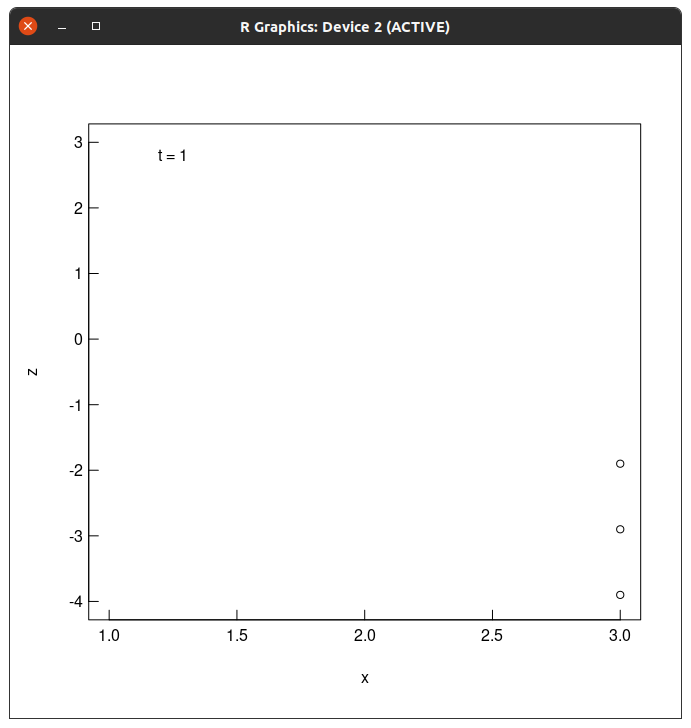
うまくいってる。
画像ファイルに出力
結果の画像をpngファイルに出力するには、次のようにすればいいとの情報を得た。
まず、これを最初のほうに書く。
png(filename="%04d.png",width=960,height=960,units="px",res=192)
すると、 plot() 関数の結果が画面でなくファイルに書き込まれるらしい。
ファイル名は 0000.png 0001.png 0002.png ... と連番でつけられる。
そして、最後にこれを書く。
graphics.off()
画像ファイルを閉じる関数らしい。
実行!
実行すると、201個! もpngファイルが作られた。
中身は全部画面出力と同じ画像(1個の時刻の分が1個のpngファイルになる)で、どうやらうまくいってる模様。
マウスでフォルダを開き、画像ファイルをクリックして開くと画像ビューアで見られるが、そのウインドウの上でPgUpかPgDnキーを押し続けると、パラパラ漫画の要領でスムーズにアニメーションして見えた。
これだと好きなところで止めたり、進んだり戻ったりして観察できるのでとても便利だ。
こいつはいい。
AVI動画に変換
ふつうに再生される動画ファイルもできたほうが便利だと思い、AVIファイルにしてみた。
変換の仕方は
% ffmpeg -i %04d.png -vcodec mjpeg three_balls.avi
簡単でびっくりしちゃった。
で、こんな感じ。
わざわざaviを再びgifに変換してアップした。どうも気持ち悪い手順だが。
ffmpeg でpngの束を直接アニメーションgifに変換する方法も見つけたんだけど、今回はpngの枚数が多すぎるせいなのか、なぜか思ったようなgifにならなかった。
いろいろな多体系の運動を解いてみる
長くなったので、別記事で。
次の記事
祝、初記事投稿
でした。ちょっといまどきどきしてます。
記事のお作法とかまだわかってなくてすみません。
それでも、どこかで誰かのお役にたったりしたら泣くほど嬉しいです。
追記
2021/04/01
rv などを マトリックスとしていたのを、データフレームとするように修正しました。
2022/02/03
次の記事へのリンクを貼りました。