構造的トピックモデルとは何か

構造的トピックモデルは、任意の共変量を加えることができるトピックモデルの発展形である。二種類の共変量があり、各トピックがドキュメントにどの程度寄与するのかに関するtopical prevalence covariatesとトピックの内における語の用いられ方の違いに関するtopical content covariatesがある。共変量を加えない場合、モデルは相関トピックモデルとなる。

stmによる構造的トピックモデル

構造的トピックモデルはRによるパッケージstmが開発されている。
まずは、パッケージをダウンロードする。

library(tidyverse)
library(dplyr)
library(tm)
library(stm)
library(wordcloud)
library(igraph)

データセットはKaggleにあるトランプとバイデンのツイートデータセットを用いる。

stmは次のようなデータ構造を必要とする。

単語文書行列
単語のベクトル
メタデータの行列

trump_tweet_df <- read.csv("/content/trumptweets.csv")
biden_tweet_df <- read.csv("/content/JoeBidenTweets.csv")

trump_tweet_df$type <- " Donald Trump"
biden_tweet_df$type <- "Joe Biden"
trump_tweet_df <- trump_tweet_df %>% rename("tweet" = content) 
biden_tweet_df <- biden_tweet_df %>% rename("date" = timestamp)
tweet_df <- rbind(trump_tweet_df[c("tweet", "type", "date")], biden_tweet_df[c("tweet", "type", "date")])
#メンションとurlを省く
tweet_df <- tweet_df %>% filter(!grepl("@", tweet)) %>% filter(!grepl("http", tweet))
tweet_df <- cbind(tweet_df[c("tweet", "type")], strftime(tweet_df$date, format = "%Y%m%d")) 
colnames(tweet_df) <- c("tweet", "type", "date")

processed <- textProcessor(tweet_df$tweet, metadata = tweet_df)

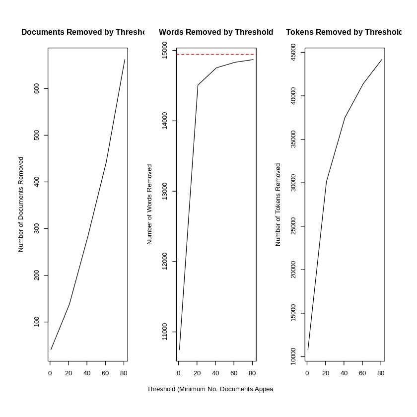
plotRemoved関数で、閾値に対して取り除かれる語の数がわかる。これを見ながら、lower.threshとupper.threshで取り除く単語数の下限と上限を設定することができる。

plotRemoved(processed$documents, lower.thresh = seq(1, 100, by = 20))
out <- prepDocuments(processed$documents, processed$vocab, processed$meta, lower.thresh = 3)

searchK関数でトピック数の探索ができる。引数Kがトピック数であるため、探索したいトピック数を格納したベクトルを与える。init.typeはinitalizetionのタイプを指定する引数である。

stm_searchk <- searchK(out$documents, vocab = out$vocab, K = c(5,10,15,20,25,30), max.em.its = 75, data = out$meta, init.type = "Spectral", content =~ type, prevalence =~ type)
plot(stm_searchk, type = "summary", xlim = c(0, 0.3))

held-out likelihoodと(共変量を設定していると出ない)semantic coherenceは高いほど、residualsと lower boundは低いほどいい指標である。

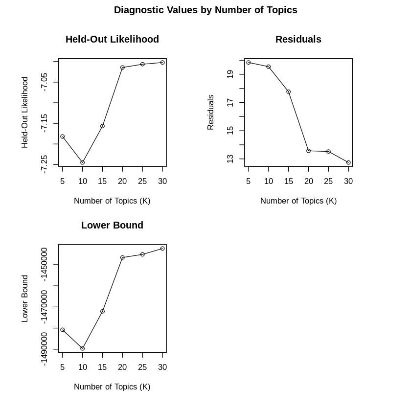
判断が難しいが、ここではトピック数を20に設定してみる。

n_topic <- 20
stm_fit <- stm(documents = out$documents, vocab = out$vocab, K = n_topic, max.em.its = 75, data = out$meta, init.type = "Spectral",  content =~ type, prevalence =~ type)
plot(stm_fit, type = "summary", xlim = c(0, 0.3))

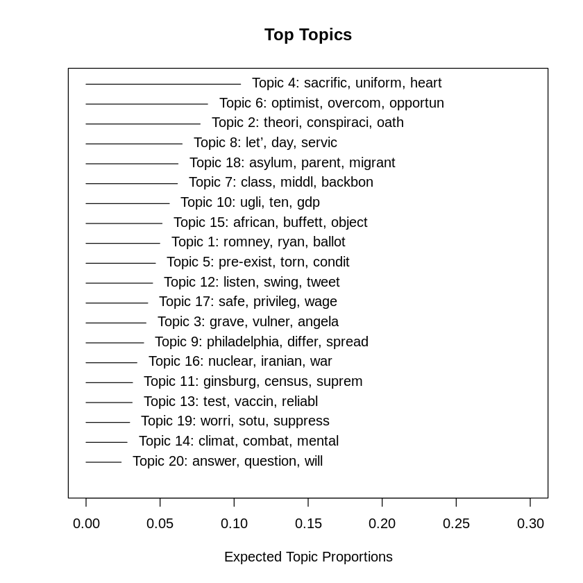
トピックを確認する

トピック名を決めるうえでは、labelTopics関数を用いるのが便利である。

labelTopics(stm_fit, c(16))
"""Topic Words:
Topic Words:
 Topic 16: nuclear, iranian, war, iran’, reckless, europ, internet 
 
 Covariate Words:
 Group  Donald Trump: pathet, correct, various, recent, origin, insid, obvious 
 Group Joe Biden: biden-harri, families”, –vp, well-connect, repay, low-incom, alongsid 
 
 Topic-Covariate Interactions:
 Topic 16, Group  Donald Trump: generat, dreamer, amp, survivor, jimmi, abil, what 
 Topic 16, Group Joe Biden: occasion, scientist, strive, indict, rocket, daili, episod  """

ワードクラウドを出力することもできる。

for(i in 1:n_topic){
    cloud(stm_fit, topic = i, scale = c(10, 1))
}

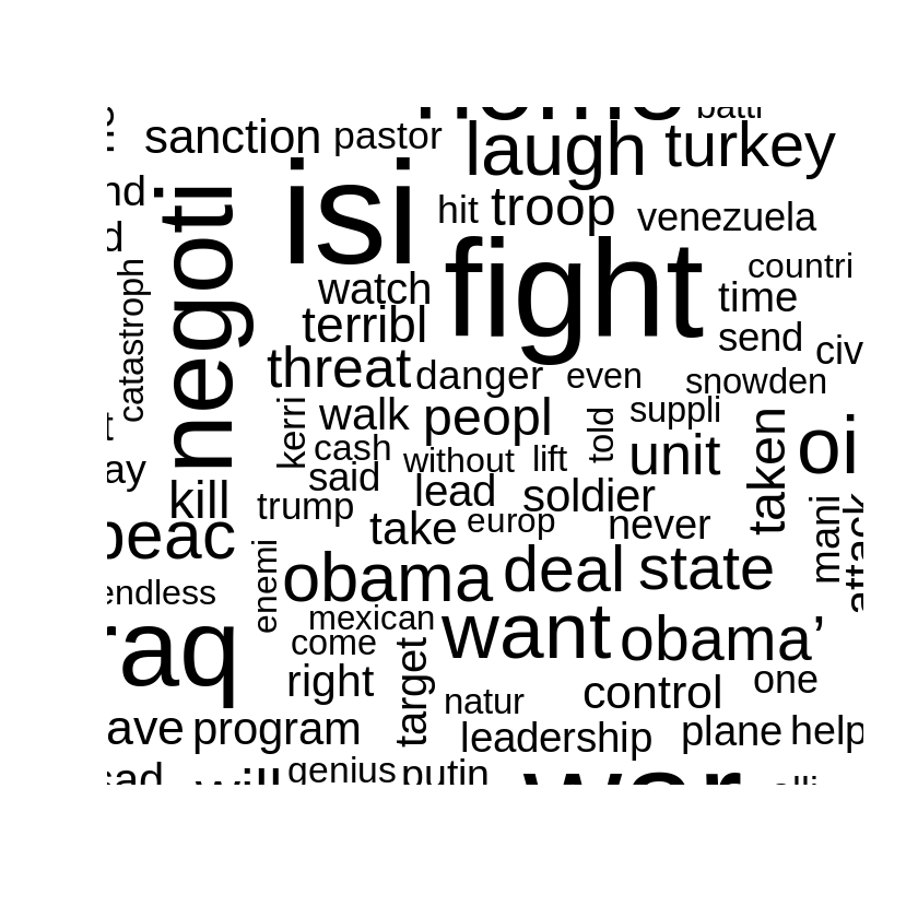
トピック16はfight, soldier, killという語があることから、戦争に関するトピックであることが分かる。

内容共変量

内容共変量(content covariates)を入れているため、トランプとバイデンでトピックにおける言葉遣いがどのように違うのかを見てみることができる。

for (i in 1:n_topic) {
    plot(stm_fit, type = "perspectives", topics = i)
}

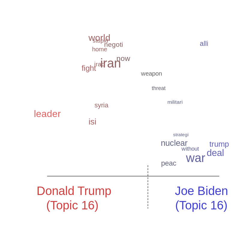
トピック16ではトランプはiran, iraq, fightという語を用いて、バイデンはnuclear, warという語を用いるのも興味深い。色はアルファベット順で決まるので、TrumpとBidenにするとTrumpが青、Bidenが赤になる。

普及共変量

普及共変量(prevalence covariates)を入れているので、トピック間の相関についても見ていくことができる。

mod.out.corr <- topicCorr(stm_fit)
plot(mod.out.corr)

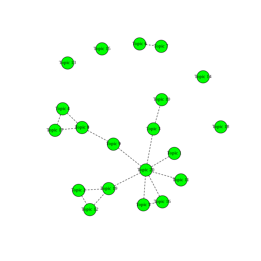
戦争のトピック16と相関があるのは、トピック5とトピック20であることが見て取れる。

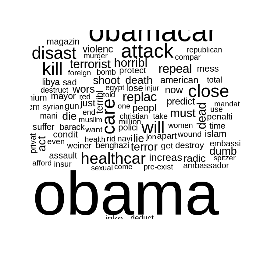
トピック5は、terrorist, kill, violence, gunがあることからテロに関するトピックであることが推測される。

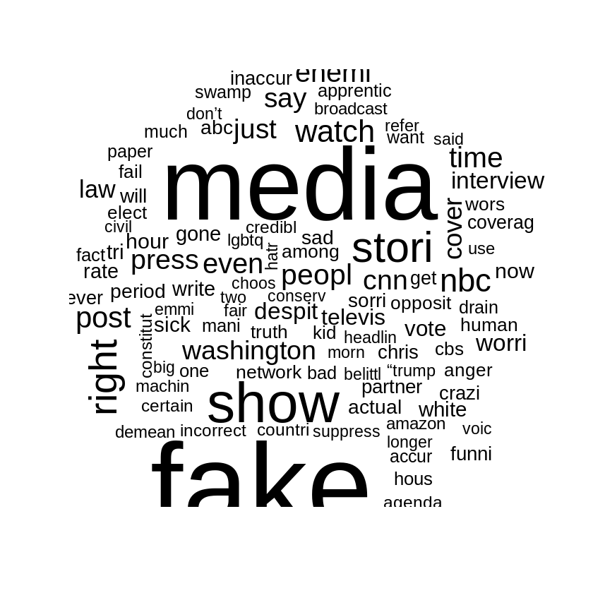
トピック20はmdeia, press, interviewの語があることから報道に関するトピックであると考えられる。

戦争トピックが、テロに関するトピックや報道に関するトピックに相関があることは、直感的にも合っているので、うまく推論できていると考えられる。

トランプとバイデンのトピックにおける言葉遣いの違いは何か?: stmによる構造的トピックモデルの紹介

構造的トピックモデルとは何か

stmによる構造的トピックモデル

トピックを確認する

内容共変量

普及共変量

参考文献