ステーキ内部の熱伝導を数値計算する（物理演算超入門）

旨い肉が食べたい（はじめに）

画像：グルナビ

• ステーキやローストビーフの焼き加減は簡単に見えて奥が深く、素人には肉を切ってみるまで内部の状態が分かりません。
• 絶妙な焼き加減を求めて試行錯誤するのもいいですが、肉がもったいないので、数値計算で推定・可視化してみましょう。
• わずか80行で役に立つプログラムが書けるので、物理演算入門に最適（！？）

問題設定

• ラップトップでも短時間で計算できるように、今回解くのは一次元熱拡散方程式です。一次元なので、平面、円柱、球の3つが取り扱えます。また、オーブンのように、肉が両面（全面）から同時に加熱されることを考えます。

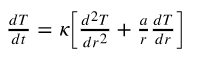
• この問題を解くための数式は以下の通りで、温度の時間変化（左辺）が温度の空間分布（右辺）で説明されています。Tは温度、tは時間、κは熱拡散係数、rは中心からの距離、aは0から2までの値を取る形状ファクターで（平面のとき0、円柱のとき1、球のとき2）、最小辺長が同じ肉ならば形状ファクターが大きいほど（肉の長辺が小さいほど）早く火が通ります。
  

• 説明で使うための物理的なパラメータを決め打ちしましょう。

  • 熱拡散係数 κ = 1.1E-7 m2/s （牛肉）
  • 初期温度 10℃ （冷蔵庫から出したて）
  • 境界温度 100℃ （表面の水分が沸騰しジュージューと音を立てている状態）
  • 肉の厚み（最小辺） 4cm
  • 肉の形状ファクター a = 0 （平面）

準備

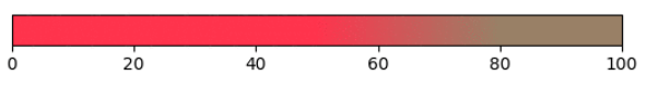
• 気分を盛り上げるために牛肉らしいカラースキームを用意しておきます。

    dict_beef = {'red':   ((0.0, 1.0, 1.0), (0.5, 1.0, 1.0), (0.8, 0.6, 0.6), (1.0, 0.6, 0.6)),
                 'green': ((0.0, 0.2, 0.2), (0.5, 0.2, 0.2), (0.8, 0.5, 0.5), (1.0, 0.5, 0.5)),
                 'blue':  ((0.0, 0.3, 0.3), (0.5, 0.3, 0.3), (0.8, 0.4, 0.4), (1.0, 0.4, 0.4)) }
    cm_beef = LinearSegmentedColormap('beef', dict_beef)

これを0から100度の範囲で表示したものがこちらです。50度から80度にかけて牛肉が変性していくのがイメージできますか？
なお、この例では、いったん加熱された肉は冷めることがないので、現在温度＝過去最高温度になります。

方程式の数値解法

• 物理演算と聞くと難しそうですが、コンセプトは簡単です：
  1. 空間を Δr 毎の格子に区切り、各格子に初期温度を与えます。
  2. 現在の T の分布から、右辺を用いて時間変化率を求めます。
  3. それを用いて、Δt だけ未来の状態を推定します。
  4. 2と3を繰り返します。

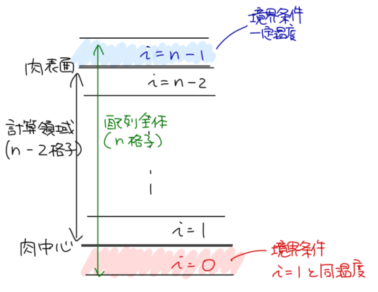
1. 格子の設計と境界条件の取り扱い

• 両面加熱のため反転対称になるので、片側半分だけ計算しておいてプロットの段階で両側を計算した風に見せます。
• 演算領域temperature[1:-1]の外側に架空の格子temperature[0], temperature[-1]を設けて、境界条件を与えます。

2. 時間変化率の計算（空間微分）

• 各格子について、二階微分 d2T/dr2 と一階微分 dT/dr が必要になります。これらは、それぞれ以下のように近似できます。
  • d2T/dr2 = [T(r+Δr) - 2T(r) + T(r-Δr)] / (Δr**2)
  • dT/dr = [T(r+Δr) - T(r-Δr)] / (2Δr)

def time_derivative(temperature):
    r = np.linspace(0, rmax, nr, endpoint=True) - delta_r / 2
    dtdt = np.empty((nr,))
    dtdt[-1] = 0.0     # outer boundary condition (constant)
    dtdt[1:-1] = kappa * \
        ((temperature[2:] - 2.0 * temperature[1:-1] + temperature[0:-2]) / (delta_r * delta_r) \
         + a_factor / r[1:-1] * (temperature[2:] - temperature[0:-2]) / (2 * delta_r))
    dtdt[0] = dtdt[1]  # inner boundary condition temperature[0] = temperature[1]
    return dtdt

3. 次のステップの状態推定（時間積分）

• 現在の T の値に温度変化率 dT/dt と時間差分 Δt の積を足した値が次のステップの T の値です。

        dtdt = time_derivative(temperature)
        temperature[:] = temperature[:] + delta_t * dtdt[:]

可視化と結果

• 連番の PNG を大量に書いて、最後に imagemagick でアニメ gif 化するのが簡単です（コード全容参照）。
• この例では20分でミディアム、30分でウェルダンという感じでしょうか。

コード全容

#!/usr/bin/env python3

import numpy as np
import os
from matplotlib import pyplot as plt
from matplotlib.colors import LinearSegmentedColormap

kappa = 1.1e-7         # [m2/s]
temp_init = 10.0       # [C]
temp_boundary = 100.0  # [C]
rmax = 4 * 0.01 * 0.5  # half-diameter [m]
a_factor = 0.0         # 0 for slab, 1 for cylinder, 2 for sphere

tmax = 100.0 * 1.5 * (rmax / 0.005) ** 2
delta_t = 0.01 * (rmax / 0.005) ** 2
delta_r = rmax / 25.0
nr = int(rmax / delta_r)
nstep = int(tmax / delta_t)
plot_intvl = 200

def main():
    os.system("mkdir -p img")
    temperature = np.full((nr,), temp_init)
    temperature[-1] = temp_boundary  # outer boundary condition

    for i in range(nstep):
        if (i % plot_intvl == 0):
            plot_snap(temperature, i)
        dtdt = time_derivative(temperature)
        temperature[:] = temperature[:] + delta_t * dtdt[:]

    os.system("convert -delay 15 -layers OptimizeTransparency -loop 0 ./img/*.png ./img/all.gif")
    os.system("rm -f img/*.png")

def time_derivative(temperature):
    r = np.linspace(0, rmax, nr, endpoint=True) - delta_r / 2
    dtdt = np.empty((nr,))
    dtdt[-1] = 0.0     # outer boundary condition (constant)
    dtdt[1:-1] = kappa * \
        ((temperature[2:] - 2.0 * temperature[1:-1] + temperature[0:-2]) / (delta_r * delta_r) \
         + a_factor / r[1:-1] * (temperature[2:] - temperature[0:-2]) / (2 * delta_r))
    dtdt[0] = dtdt[1]  # inner boundary condition temperature[0] = temperature[1]
    return dtdt

def plot_snap(temperature, i):
    # save a snapshot at i-th step
    dict_beef = {'red':   ((0.0, 1.0, 1.0), (0.5, 1.0, 1.0), (0.8, 0.6, 0.6), (1.0, 0.6, 0.6)),
                 'green': ((0.0, 0.2, 0.2), (0.5, 0.2, 0.2), (0.8, 0.5, 0.5), (1.0, 0.5, 0.5)),
                 'blue':  ((0.0, 0.3, 0.3), (0.5, 0.3, 0.3), (0.8, 0.4, 0.4), (1.0, 0.4, 0.4)) }
    cm_beef = LinearSegmentedColormap('beef', dict_beef)

    xdim = 10  # horizontal dimension for visualization
    data = np.zeros((nr*2,xdim))
    for k in range(xdim):  # plot both sides mirrored
        data[0:nr,   k] = temperature[::-1]
        data[nr:2*nr,k] = temperature
    fig, ax = plt.subplots(1)
    plt.imshow(data, cmap=cm_beef, interpolation="bilinear", aspect=0.1)
    plt.clim(0, 100.0)
    plt.tick_params(axis="x", which="both", bottom="off", top="off", labelbottom="off")
    plt.tick_params(axis="y", which="both", left="off", right="off", labelleft="off")
    plt.colorbar(orientation="horizontal")

    levels = np.arange(0, 100, 10)
    extent = (-0.5, xdim-0.5, 0, nr*2-1)
    map2 = ax.contour(data, levels, colors="w", extent=extent)
    ax.clabel(map2, fmt="%02d", colors="w")

    plt.title("[%d cm, init %i deg, boundary %i deg] t = %isec" %
              (rmax*2*100, temp_init, temp_boundary, i*delta_t))
    plt.savefig("./img/%06i.png" % i)
    plt.close()

main()