GeForce GTX 1070 (8GB)
ASRock Z170M Pro4S [Intel Z170chipset]
Ubuntu 16.04 LTS desktop amd64
TensorFlow v1.1.0
cuDNN v5.1 for Linux
CUDA v8.0
Python 3.5.2
IPython 6.0.0 -- An enhanced Interactive Python.
gcc (Ubuntu 5.4.0-6ubuntu1~16.04.4) 5.4.0 20160609
GNU bash, version 4.3.48(1)-release (x86_64-pc-linux-gnu)
学習コードv0.1 http://qiita.com/7of9/items/5819f36e78cc4290614e
http://qiita.com/7of9/items/35e51bd6f387c26c8009
の続き。
概要
This article is related to ADDA (light scattering simulator based on the discrete dipole approximation).
- TFRecordsを読込んで学習する
- input: 5 nodes
- output: 6 nodes
- サンプル数: 223,872
- 学習データ: ADDAにより計算した値
- #input
- x,y,z: dipole position
- refractive index: real and imaginary part
- #output
- initial values for linear equation solution for (x,y,z),(real,imaginary)
5次元補間を学習させようとしている。
上記のパラメータのうち、refractive index は以下の値を用いた。
real part [1.45, 1.5, 1.33, 1.4]
imaginary part [0.001, 0.050000001, 0.029999999, 0.1, 0.0099999998, 9.9999997e-05]
ネットワークはhidden layerが30x100x100の3層とした。
学習
学習データ
TensorFlow > 複数のTFRecordsファイルを1つにまとめる v0.1,v0.2
で作成したcombined_IntField-Y_170722.tfrecordsを以下のようにリンクしておく。
$ ln -fs combined_IntField-Y_170722.tfrecords LN-IntField-Y_170722.tfrecords
学習コード v0.8
import numpy as np
import tensorflow as tf
import tensorflow.contrib.slim as slim

"""
v0.8 Jul. 28, 2017
  - change batch size from [4] to [2]
  - change learning rate from [0.0001] to [0.001]
v0.7 Jul. 28, 2017
  - change learning rate from [0.001] to [0.0001]
v0.6 Jul. 27, 2017
  - increase step from [1,000,000] to [3,000,000]
v0.5 Jul. 25, 2017
  - change network to [30,100,100]
  - increase step to [1,000,000]
v0.4 Jul. 23, 2017
  - increase step from [90000] to [270000]
v0.3 Jul. 22, 2017
  - output model variables
v0.2 Jul. 22, 2017
  - increase step from [30000] to [90000]
  - change [capacity]
v0.1 Jul. 22, 2017
  - increase network structure from [7,7,7] to [100,100,100]
  - increase dimension of [input_ph], [output_ph]
  - alter read_and_decode() to treat 5 input-, 6 output- nodes
  - alter [IN_FILE] to the symbolic linked file

  :reference: [learnExr_170504.py] to expand dimensions to [input:3,output:6]

=== branched from [learn_sineCurve_170708.py] ===
v0.6 Jul. 09, 2017
  - modify for PEP8
  - print prediction after learning
v0.5 Jul. 09, 2017
  - fix bug > [Attempting to use uninitialized value hidden/hidden_1/weights]
v0.4 Jul. 09, 2017
  - fix bug > stops only for one epoch
    + set [num_epochs=None] for string_input_producer()
  - change parameters for shuffle_batch()
  - implement training
v0.3 Jul. 09, 2017
  - fix warning > use tf.local_variables_initializer() instead of
       initialize_local_variables()
  - fix warning > use tf.global_variables_initializer() instead of
       initialize_all_variables()
v0.2 Jul. 08, 2017
  - fix bug > OutOfRangeError (current size 0)
    + use [tf.initialize_local_variables()]
v0.1 Jul. 08, 2017
  - only read [.tfrecords]
    + add inputs_xy()
    + add read_and_decode()
"""

# codingrule: PEP8

IN_FILE = 'LN-IntField-Y_170722.tfrecords'


def read_and_decode(filename_queue):
    reader = tf.TFRecordReader()
    _, serialized_example = reader.read(filename_queue)
    features = tf.parse_single_example(
        serialized_example,
        features={
           'xpos_raw': tf.FixedLenFeature([], tf.string),
           'ypos_raw': tf.FixedLenFeature([], tf.string),
           'zpos_raw': tf.FixedLenFeature([], tf.string),
           'mr_raw': tf.FixedLenFeature([], tf.string),
           'mi_raw': tf.FixedLenFeature([], tf.string),
           'exr_raw': tf.FixedLenFeature([], tf.string),
           'exi_raw': tf.FixedLenFeature([], tf.string),
           'eyr_raw': tf.FixedLenFeature([], tf.string),
           'eyi_raw': tf.FixedLenFeature([], tf.string),
           'ezr_raw': tf.FixedLenFeature([], tf.string),
           'ezi_raw': tf.FixedLenFeature([], tf.string),
        })
    xpos_raw = tf.decode_raw(features['xpos_raw'], tf.float32)
    ypos_raw = tf.decode_raw(features['ypos_raw'], tf.float32)
    zpos_raw = tf.decode_raw(features['zpos_raw'], tf.float32)
    mr_raw = tf.decode_raw(features['mr_raw'], tf.float32)
    mi_raw = tf.decode_raw(features['mi_raw'], tf.float32)
    exr_raw = tf.decode_raw(features['exr_raw'], tf.float32)
    exi_raw = tf.decode_raw(features['exi_raw'], tf.float32)
    eyr_raw = tf.decode_raw(features['eyr_raw'], tf.float32)
    eyi_raw = tf.decode_raw(features['eyi_raw'], tf.float32)
    ezr_raw = tf.decode_raw(features['ezr_raw'], tf.float32)
    ezi_raw = tf.decode_raw(features['ezi_raw'], tf.float32)

    xpos_org = tf.reshape(xpos_raw, [1])
    ypos_org = tf.reshape(ypos_raw, [1])
    zpos_org = tf.reshape(zpos_raw, [1])
    mr_org = tf.reshape(mr_raw, [1])
    mi_org = tf.reshape(mi_raw, [1])
    exr_org = tf.reshape(exr_raw, [1])
    exi_org = tf.reshape(exi_raw, [1])
    eyr_org = tf.reshape(eyr_raw, [1])
    eyi_org = tf.reshape(eyi_raw, [1])
    ezr_org = tf.reshape(ezr_raw, [1])
    ezi_org = tf.reshape(ezi_raw, [1])
    # input
    wrk = [xpos_org[0], ypos_org[0], zpos_org[0], mr_org[0], mi_org[0]]
    inputs = tf.stack(wrk)
    # output
    wrk = [exr_org[0], exi_org[0],
           eyr_org[0], eyi_org[0],
           ezr_org[0], ezi_org[0]]
    outputs = tf.stack(wrk)
    return inputs, outputs


def inputs_xy():
    filename = IN_FILE
    filequeue = tf.train.string_input_producer(
        [filename], num_epochs=None)

    in_org, out_org = read_and_decode(filequeue)
    return in_org, out_org

in_orgs, out_orgs = inputs_xy()
batch_size = 2  # [4]
# Ref: cifar10_input.py
min_fraction_of_examples_in_queue = 0.2  # 0.4
NUM_EXAMPLES_PER_EPOCH_FOR_TRAIN = 223872  # 223872 or 9328
min_queue_examples = int(NUM_EXAMPLES_PER_EPOCH_FOR_TRAIN *
                         min_fraction_of_examples_in_queue)
cpcty = min_queue_examples + 3 * batch_size
in_batch, out_batch = tf.train.shuffle_batch([in_orgs, out_orgs],
                                             batch_size,
                                             capacity=cpcty,
                                             min_after_dequeue=batch_size)

input_ph = tf.placeholder("float", [None, 5])
output_ph = tf.placeholder("float", [None, 6])  # [6]

# network
hiddens = slim.stack(input_ph, slim.fully_connected, [30, 100, 100],
                     activation_fn=tf.nn.sigmoid, scope="hidden")
prediction = slim.fully_connected(hiddens, 6,
                                  activation_fn=None, scope="output")
loss = tf.contrib.losses.mean_squared_error(prediction, output_ph)

train_op = slim.learning.create_train_op(loss, tf.train.AdamOptimizer(0.001))

init_op = [tf.global_variables_initializer(), tf.local_variables_initializer()]

with tf.Session() as sess:
    sess.run(init_op)
    coord = tf.train.Coordinator()
    threads = tf.train.start_queue_runners(sess=sess, coord=coord)

    try:
        for idx in range(3000000):  # 1000000
            inpbt, outbt = sess.run([in_batch, out_batch])
            _, t_loss = sess.run([train_op, loss],
                                 feed_dict={input_ph: inpbt, output_ph: outbt})
            if (idx + 1) % 100 == 0:
                print("%d,%f" % (idx+1, t_loss))
    finally:
        coord.request_stop()

    # output the model
    model_variables = slim.get_model_variables()
    res = sess.run(model_variables)
    np.save('model_variables_170722.npy', res)

    coord.join(threads)
学習コードバッチ処理スクリプト(bash)
1つの処理がだいたい30分程度かかる。処理ごとに日時のプリフィックスを結果ファイル名に付加して、複数回実行するようなスクリプトを用意した。
# !/usr/bin/env bash

trap exit SIGINT  # to exit for Ctrl+c


for dd in $(seq 1 8)
do
	PREFIX=$(date "+%y%m%d_t%H%M")
	echo $PREFIX
	python3 learn_mr_mi_170722.py > log_learn.$PREFIX
	mv model_variables_170722.npy model_variables_170722.npy.$PREFIX
done
以下のように使用することで、8回までの処理が行われる。
bash group_run_170727_exec
lossの経過
logファイル
上記のgroup_run_170727_execにより以下のようなファイルがそれぞれの処理開始日時で作成される。
(2017/07/28 23:11に処理開始)
log_learn.170728_t2311 : ログファイル
model_variables_170722.npy.170728_t2311 : ネットワークファイル
これらのファイルを作成したディレクトリ(例. RES_170729_t0744)に移動しておく。
ディレクトリはlearning rateやbatch sizeなどのパラメータを変えた時に新規ディレクトリを作ることで、パラメータの混在を避ける。
loss経過の表示コード
lossの経過はそのままでは振幅が大きく、複数の結果を比較しにくい。
移動平均処理を行い、比較をできるようにした。
TensorFlow > lossの経過の可視化 > moving average処理 | 複数プロットの対応
Jupyter code.
%matplotlib inline

# learning [Exr,Exi,Eyr,Eyi,Ezr,Ezi] from ADDA
# Jul. 28, 2017

import numpy as np
import matplotlib.pyplot as plt


def moving_average(a, n=3) :
    # from
    # https://stackoverflow.com/questions/14313510/how-to-calculate-moving-average-using-numpy
    ret = np.cumsum(a, dtype=float)
    ret[n:] = ret[n:] - ret[:-n]
    return ret[n - 1:] / n


def add_lineplot(filepath, ax1, alabel):
    data1 = np.loadtxt(filepath, delimiter=',')
    input1 = data1[:,0]
    output1 = data1[:,1]

    # moving average
    NUM_AVERAGE = 50
    output1 = moving_average(output1, n=NUM_AVERAGE)
    for loop in range(NUM_AVERAGE - 1):
        output1 = np.append(output1, 1e-7)  # dummy

    ax1.plot(input1, output1, label=alabel)

fig = plt.figure(figsize=(10,10),dpi=200)
ax1 = fig.add_subplot(2,1,1)
ax1.grid(True)
ax1.set_xlabel('step')
ax1.set_ylabel('loss')
ax1.set_yscale('log')
ax1.set_xlim([0, 3000000])
ax1.set_ylim([1e-5, 1.0])

# --- learning rate=0.001, batch_size=4
FILE_PATH1 = 'RES_170728_t0716//log_learn.170727_t2308'
# --- learning rate=0.0001, batch_size=4
# FILE_PATH1 = 'RES_170728_t2119/log_learn.170728_t0720'
# FILE_PATH1 = 'RES_170728_t2119/log_learn.170728_t0751'
# FILE_PATH1 = 'RES_170728_t2119/log_learn.170728_t0821'
# FILE_PATH1 = 'RES_170728_t2119/log_learn.170728_t0850'
# FILE_PATH1 = 'RES_170728_t2119/log_learn.170728_t0921'
# FILE_PATH1 = 'RES_170728_t2119/log_learn.170728_t0951'
# FILE_PATH2 = 'RES_170728_t2119/log_learn.170728_t1050'
# --- batch_size=2
FILE_PATH2 = 'RES_170729_t0744//log_learn.170728_t2311'
# --- batch_size=20
FILE_PATH3 = 'RES_170728_t2311/log_learn.170728_t2208'

# for learning rage=0.001
add_lineplot(FILE_PATH2, ax1, alabel="batch size=2")
add_lineplot(FILE_PATH1, ax1, alabel="batch size=4")
add_lineplot(FILE_PATH3, ax1, alabel="batch size=20")

ax1.legend()
結果
AdamOptimizerにてlearning rate=0.001としている。
lossの経過 > batch sizeの違い
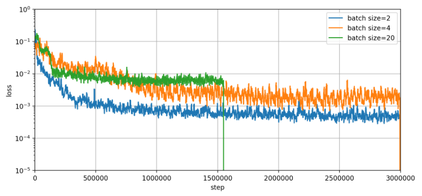
batch size=2の結果にてlossが最小になった。
処理時間は以下
- batch size=2 : 24分
- batch size=4 : 30分
- batch size=20 : 60分以上 (途中で停止)
初期値の再現
学習したネットワークを用いて
initial values for linear equation solution for (x,y,z),(real,imaginary)
の再現度を見た。
結果確認コード v0.5
Jupyter code.
import numpy as np
import tensorflow as tf
import math
import sys
import matplotlib.pyplot as plt
import matplotlib.cm as cm
import datetime

"""
v0.5 Jul. 28, 2017
    - use symbolic linked network file (LN-model_variables_170722.npy)
v0.4 Jul. 25, 2017
    - list up unique values for [arm, ami, az]
    - change if statement to exclute [amr, ami, az]
v0.3 Jul. 23, 2017
    - add [COLOR_RANGE] and (vmin, vmax) for plt.imshow()
    - fix bug > if abs() statement is the other way around
    - fix bug > TARGET_IDX.EXR..EXI is wrong
v0.2 Jul. 22, 2017
    - update calc_conv()
v0.1 Jul. 22, 2017
    - change for input incuding [mr],[mi]
=== branched from [display_TFRecords_IntField_170709.ipynb: v0.1] ===
"""

# on
#   Ubuntu 16.04 LTS
#   TensorFlow v1.1
#   Python 3.5.2
#   IPython 6.0.0 -- An enhanced Interactive Python.


def calc_sigmoid(x):
    return 1.0 / (1.0 + math.exp(-x))


def calc_conv(src, weight, bias, applyActFnc):
    wgt = weight.shape
#   print wgt # debug
    #conv = list(range(bias.size))
    conv = [0.0] * bias.size

    # weight
    #for idx1 in range(wgt[0]):
    #    for idx2 in range(wgt[1]):
    #        conv[idx2] = conv[idx2] + src[idx1] * weight[idx1, idx2]
    for   idx2 in range(wgt[1]):
        tmp_vec = weight[:,idx2] * src[:]
        conv[idx2] = tmp_vec.sum()

    # bias
    for idx2 in range(wgt[1]):
        conv[idx2] = conv[idx2] + bias[idx2]
    # activation function
    if applyActFnc:
        for idx2 in range(wgt[1]):
            conv[idx2] = calc_sigmoid(conv[idx2])
    return conv  # return list


def get_feature_float32(example, feature_name):
    wrk_raw = (example.features.feature[feature_name]
               .bytes_list
               .value[0])
    wrk_1d = np.fromstring(wrk_raw, dtype=np.float32)
    wrk_org = wrk_1d.reshape([1, -1])
    return wrk_org


def get_group_features(example):
    xpos_org = get_feature_float32(example, 'xpos_raw')
    ypos_org = get_feature_float32(example, 'ypos_raw')
    zpos_org = get_feature_float32(example, 'zpos_raw')
    mr_org = get_feature_float32(example, 'mr_raw')
    mi_org = get_feature_float32(example, 'mi_raw')
    exr_org = get_feature_float32(example, 'exr_raw')
    exi_org = get_feature_float32(example, 'exi_raw')
    eyr_org = get_feature_float32(example, 'eyr_raw')
    eyi_org = get_feature_float32(example, 'eyi_raw')
    ezr_org = get_feature_float32(example, 'ezr_raw')
    ezi_org = get_feature_float32(example, 'ezi_raw')

    pos = xpos_org[0], ypos_org[0], zpos_org[0], mr_org[0], mi_org[0]
    ex = exr_org[0], exi_org[0]
    ey = eyr_org[0], eyi_org[0]
    ez = ezr_org[0], ezi_org[0]
    return pos + ex + ey + ez


class TARGET_IDX:
    EXR, EXI = 5, 6  # real and imaginary part of Ex
    EYR, EYI = 7, 8
    EZR, EZI = 9, 10

# parameters
SIZE_MAP_X = 30  # size of the image
SIZE_MAP_Y = 30
ZOOM_X = 15.0  #
ZOOM_Y = 15.0
SHIFT_X = 15.0  # to shift the center position
SHIFT_Y = 15.0
orgmap = [[0.0 for yi in range(SIZE_MAP_Y)] for xi in range(SIZE_MAP_X)]
outmap = [[0.0 for yi in range(SIZE_MAP_Y)] for xi in range(SIZE_MAP_X)]

INP_FILE = 'LN-IntField-Y_170722.tfrecords'
# NETWORK_FILE = 'model_variables_170722.npy'
NETWORK_FILE = 'LN-model_variables_170722.npy'

pickUpZvalue = 0.23620997  # arbitrary selected
pickUpRealm = 1.45  # 1.33, 1.45  # arbitrary selected
pickUpImagm = 9.9999997e-05  # arbitrary selected

print(datetime.datetime.now())

atargetIdx = TARGET_IDX.EXR  # [set this]

model_var = np.load(NETWORK_FILE)

list_mr, list_mi, list_z = [], [], []  # debug

record_iterator = tf.python_io.tf_record_iterator(path=INP_FILE)
for record in record_iterator:
    example = tf.train.Example()
    example.ParseFromString(record)

    tpl = get_group_features(example)
    xpos_val, ypos_val, zpos_val = tpl[0:3]
    mr_val, mi_val = tpl[3:5]
    ax, ay, az = *xpos_val, *ypos_val, *zpos_val
    amr, ami = *mr_val, *mi_val
    aTarget = tpl[atargetIdx]

    if amr not in list_mr:  # debug
        list_mr.append(amr)
    if ami not in list_mi:  # debug
        list_mi.append(ami)

    if (abs(amr - pickUpRealm) > 1e-6):
        continue
    if (abs(ami - pickUpImagm) > 1e-6):
        continue

    if az not in list_z:  # debug
        list_z.append(az)

    if (abs(ami - pickUpImagm) > 1e-6):
        continue

    xidx = (SIZE_MAP_X * ax / ZOOM_X + SHIFT_X).astype(int)
    yidx = (SIZE_MAP_Y * ay / ZOOM_Y + SHIFT_Y).astype(int)

    if (xidx < 0 or xidx >= SIZE_MAP_X or
        yidx < 0 or yidx >= SIZE_MAP_Y):
        continue

    #print(az, amr, ami)
    #sys.exit()

    # input layer (5 nodes)
    inlist = (ax, ay, az, amr, ami)
    # hidden layer 1
    outdata = calc_conv(inlist, model_var[0], model_var[1], applyActFnc=True)
    # hidden layer 2
    outdata = calc_conv(outdata, model_var[2], model_var[3], applyActFnc=True)
    # hidden layer 3
    outdata = calc_conv(outdata, model_var[4], model_var[5], applyActFnc=True)
    # output layer
    outdata = calc_conv(outdata, model_var[6], model_var[7], applyActFnc=False)

    orgmap[xidx][yidx] = aTarget  # overwrite
    outmap[xidx][yidx] = outdata[atargetIdx - TARGET_IDX.EXR]
    #outmap[xidx][yidx] = 0.0  # dummy

# draw map
COLOR_RANGE = 0.5
#   original
plt.subplot(121)
figmap = np.reshape(np.array(orgmap), (SIZE_MAP_X, SIZE_MAP_Y))
plt.imshow(figmap, extent=(0, SIZE_MAP_X, 0, SIZE_MAP_Y), cmap=cm.jet, vmin=-COLOR_RANGE, vmax=COLOR_RANGE)
# plt.imshow(figmap, extent=(0, SIZE_MAP_X, 0, SIZE_MAP_Y), cmap=cm.jet)
plt.colorbar()
#   learnt
plt.subplot(122)
figmap = np.reshape(np.array(outmap), (SIZE_MAP_X, SIZE_MAP_Y))
plt.imshow(figmap, extent=(0, SIZE_MAP_X, 0, SIZE_MAP_Y), cmap=cm.jet, vmin=-COLOR_RANGE, vmax=COLOR_RANGE)
# plt.imshow(figmap, extent=(0, SIZE_MAP_X, 0, SIZE_MAP_Y), cmap=cm.jet)
plt.colorbar()

plt.show()

print(datetime.datetime.now())

print(list_mr)
print(list_mi)
print(list_z)
INP_FILEには学習対象のTFRecordsファイルを指定する。
NETWORK_FILEには学習したネットワークファイル(e.g. model_variables_170722.npy.170728_t2311)をsymbolic linkしたファイルLN-model_variables_170722.npyを使う。
INP_FILE = 'LN-IntField-Y_170722.tfrecords'
# NETWORK_FILE = 'model_variables_170722.npy'
NETWORK_FILE = 'LN-model_variables_170722.npy'
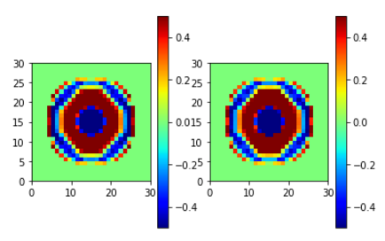
学習元と再現で比較したい値を以下のインデックスで指定する (EXR, EXI, EYR, EYI, EZR, EZI). ここでEXRはX方向の初期値の実部、EXIはX方向の初期値の虚部を表す。
atargetIdx = TARGET_IDX.EXR # [set this]
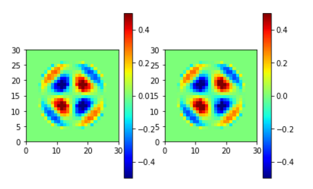
再現の結果
Zの値、refractive indexのreal, imaginary part の値は以下のように選択した。
pickUpZvalue = 0.23620997  # arbitrary selected
pickUpRealm = 1.45  # 1.33, 1.45  # arbitrary selected
pickUpImagm = 9.9999997e-05  # arbitrary selected
EXR (左が学習元、右が学習結果)
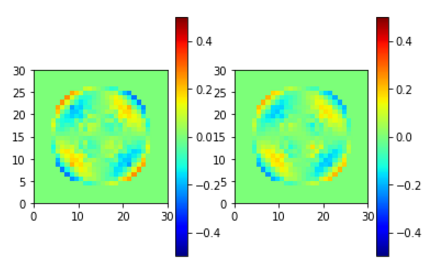
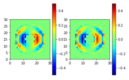
EXI (左が学習元、右が学習結果)
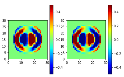
EYR (左が学習元、右が学習結果)
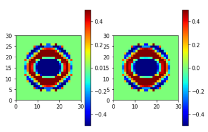
EYI (左が学習元、右が学習結果)
EZR (左が学習元、右が学習結果)
EZI (左が学習元、右が学習結果)
備考
目指していた学習が成功したように思う。
実際に対象となるADDAの初期値として使用した時、線形方程式のiteration数が実際に減るかどうかは今後の確認事項。
batch sizeについては理解が浅い。今回たまたまbatch size 2で良い結果が得られたのみ。
過学習かどうかは気になるところ。実際の用途としては、学習に用いていない中間値のrefractive indexでもうまく補間で対処してくれるかどうか。
今後確認する事項である。