先物取引におけるロールオーバーの累積リターンをモデル化してみる #Python

先物取引のモデル化

基本的に前々回と前回の続きです。

今日は先物取引の中でも定番の「金」について実際にロールオーバーから連続的なリターンを構築、予測やモデル化の一助に利用してみようという話です。

ロールオーバーとは簡単に言うと先物取引の期限が迫る契約からすぐ先もしくはだいぶ先の契約へと移行することです。取引残高の継続的な推移をモデル化するには市場や取引の様々な条件を加味しなければなりませんが、ここでは線形に推移するシンプルなモデルを考えてみます。

銘柄の選択

Gold Futures Rollover Dates 2013 を参照して適当な銘柄を選びます。執筆時点では 3/13 ですので直近で契約期限日 (Last Trade) を迎える GCJ14 と GCM14 に狙いを定めてみましょう。

ランダムウォーク

ランダムウォークで先物取引の契約をシミュレートします。

def random_walk(px, n, f):
    np.random.seed(34567)
    N = 200
    _walk = (np.random.randint(0, 200, size=N) - 100) * 0.25
    perturb = (np.random.randint(0, 20, size=N) - 10) * 0.25
    walk = _walk.cumsum()
    rng = pd.date_range(px.index[0], periods=len(px) + N, freq='B')
    near = np.concatenate([px.values, px.values[-1] + walk])
    far = np.concatenate([px.values, px.values[-1] + walk + perturb])
    prices = pd.DataFrame({n: near, f: far}, index=rng)
    return prices

ランダムウォークの関数ができました。
ではこれに Yahoo! ファイナンスのデータを渡してみましょう。

# SPY 投資信託の基準価格を S&P 500 インデックスのおよその価格として利用
px = web.get_data_yahoo('SPY')['Adj Close'] * 10
# 銘柄と契約期限日を指定
expiries = {
    'GCJ14': datetime(2014,4,28),
    'GCM14': datetime(2014,6,26)
}
expiry = pd.Series(expiries).order()

print( px.tail(5) )
# => 
# Date
# 2014-03-06    1881.8
# 2014-03-07    1882.6
# 2014-03-10    1881.6
# 2014-03-11    1872.3
# 2014-03-12    1872.8

print( expiry )
# =>
# GCJ14   2014-04-28
# GCM14   2014-06-26

prices = random_walk(px, 'GCJ14', 'GCM14')
print( prices.tail(5) )
# =>
#               GCJ14    GCM14
# 2014-10-17  1618.80  1621.05
# 2014-10-20  1634.80  1632.55
# 2014-10-21  1622.55  1623.80
# 2014-10-22  1638.55  1639.30
# 2014-10-23  1637.55  1638.30

重み付け

次に重み付けを計算するモデルを構築します。コードはオライリー本そのままです。

def get_roll_weights(start, expiry, items, roll_periods=5):
    dates = pd.date_range(start, expiry[-1], freq='B')
    weights = pd.DataFrame(np.zeros((len(dates), len(items))),
                        index=dates, columns=items)
    prev_date = weights.index[0]
    for i, (item, ex_date) in enumerate( expiry.iteritems() ):
        if i < len(expiry) - 1:
            weights.ix[prev_date:ex_date - pd.offsets.BDay(), item] = 1
            roll_rng = pd.date_range(end=ex_date - pd.offsets.BDay(),
                                     periods=roll_periods + 1, freq='B')
            decay_weights = np.linspace(0, 1, roll_periods + 1)
            weights.ix[roll_rng, item] = 1 - decay_weights
            weights.ix[roll_rng, expiry.index[i + 1]] = decay_weights
        else:
            weights.ix[prev_date:, item] = 1
        prev_date = ex_date
    return weights

連続的なリターンの算出

最後にこれらの関数を利用して連続的なリターンインデックスを求めます。

weights = get_roll_weights('3/11/2014', expiry, prices.columns)

sample_prices  = prices.ix['2014-04-17' : '2014-04-28']
sample_weights = weights.ix['2014-04-17' : '2014-04-28']
sample = sample_prices * sample_weights

# データフレームを新しく構築
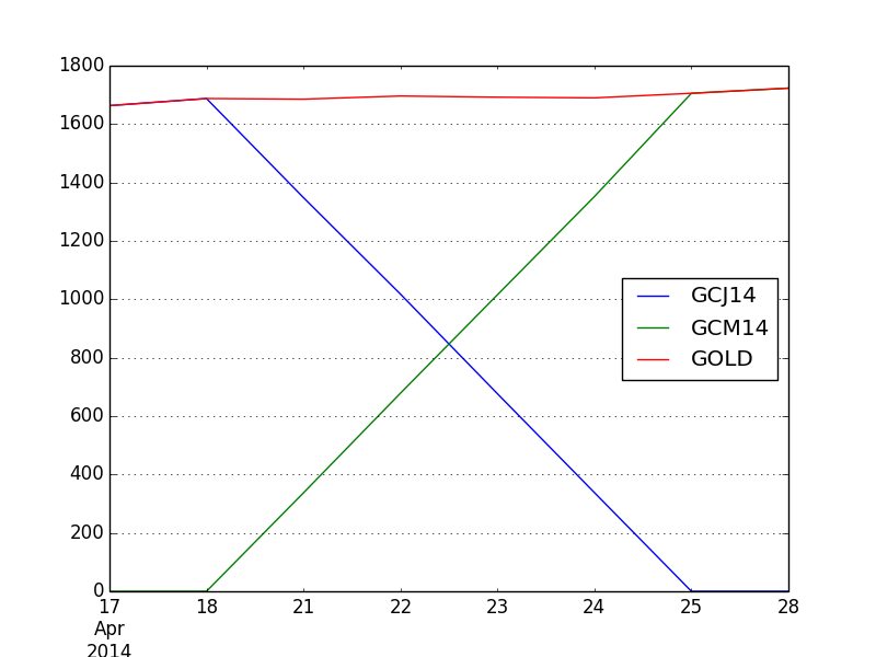
result = pd.DataFrame({'GCJ14': sample['GCJ14'], 'GCM14': sample['GCM14'], 'GOLD': sample['GCJ14'] + sample['GCM14'] })

# ロールオーバーされた先物取引のリターンを得る
print( result )
# =>
#               GCJ14    GCM14     GOLD
# 2014-04-17  1663.30     0.00  1663.30
# 2014-04-18  1687.55     0.00  1687.55
# 2014-04-21  1348.24   337.16  1685.40
# 2014-04-22  1017.78   678.42  1696.20
# 2014-04-23   676.62  1015.53  1692.15
# 2014-04-24   338.01  1351.84  1689.85
# 2014-04-25     0.00  1705.55  1705.55
# 2014-04-28     0.00  1723.05  1723.05

株式ポートフォリオを分析するのはこれくらいにして次回以降はまた別の分野に応用していきます。

参考

Pythonによるデータ分析入門――NumPy、pandasを使ったデータ処理
http://www.oreilly.co.jp/books/9784873116556/