画像処理ライブラリに頼らず、行列演算だけで自分なりにアンチエイリアス直線を描くお話。Pythonistaでも可能
独自研究!?
ブレゼンハムのアルゴリズムを読んでいると、Xiaolin Wuのアルゴリズムなるものがあったり、ほかにもGupta-Sproullのアルゴリズムがあった。しかし、行列計算を使えば、もうちょっとがんばれそうと思った。
見つからなかったから独自研究と銘打ったが、独自性はないと思う。(要するに再発明)
コンセプト
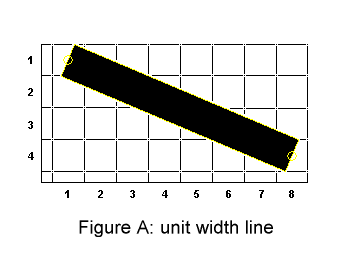
ここから拝借
上の図は太さ1の直線が、様々なピクセルにまたがっていることを示している。
このまたがった面積に応じた濃さを各ピクセルに与えたい。
状況設定
手書き失礼
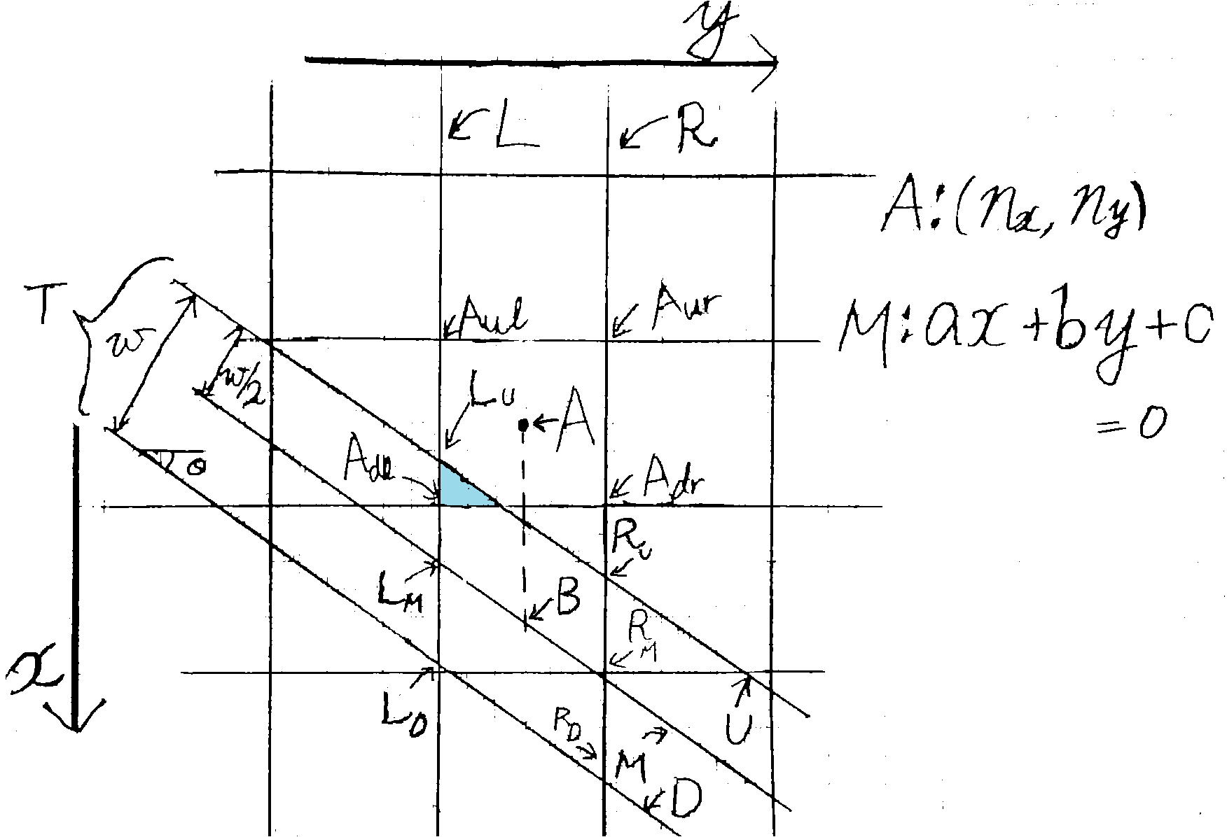
上図は、ピクセルの中に直線が引かれた様子を示すものである。
すなわち、マス目がピクセルを示し、斜めにひかれた3本の直線は、一本の太い直線T(真ん中の直線Mは中央線)を示す。
中央が点A$(n_x,n_y)$であるピクセルと、太さが$w/2$の直線T$ax+by+c=0$を考える。ただし、$a\geq-b\geq0,a>0$である。また、直線の傾き$\theta = -\arctan\frac{b}{a}$である。
このピクセルは四隅の点はそれぞれ左上$A_{ul}(n_x-0.5,n_y-0.5)$,
右上$A_{ur}(n_x-0.5,n_y+0.5)$、
左下$A_{dl}(n_x+0.5,n_y-0.5)$、
右下$A_{dr}(n_x+0.5,n_y+0.5)$である。
一方の太い直線Tについては、上限を示すU、下限を示すD、中央を走るMの三本が図中に示されている。
中央線から上下の線へはどちらも距離$w/2$だけ離れており、全体の太さは$w$になる。
また、A中心のピクセルの左端、右端と一致する直線はそれぞれL,Rであり、それらがどの直線と交わるかによってL,Rという文字の下付き文字が変わる。
問題設定
上の状況において、ピクセルAと、平行四辺形B$L_UR_UR_DL_D$(点BはAのx軸正方向にある直線M上の点)の共通部分(水色)の面積Sを求める。
S_Xの定義
$t=(Bのx座標)-(A_{ul}A_{ur}のx座標)$をとしたとき、線分$A_{ul}A_{ur}$より下(x軸正方向)にある図形$X$の面積を$S_X(t)$とすると(上から下へ図形を平行移動させているイメージ)
S=S_B(t)-S_B(t-1)
となる。第二項は線分$A_{dl}A_{dr}$より下になった部分の面積である。
よって、$S_B(t)$を求めればよい。
平行四辺形Bの分解
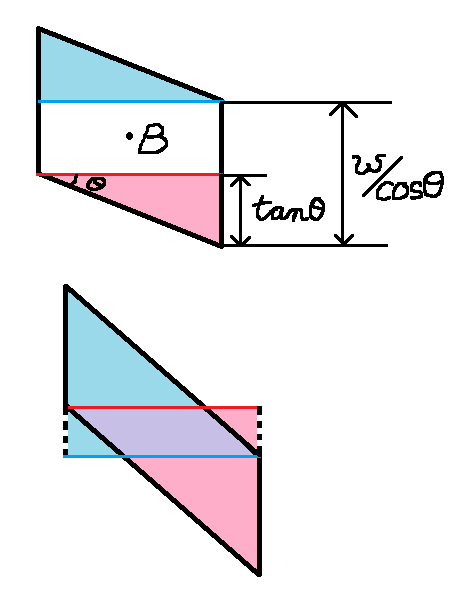
平行四辺形B$L_UR_UR_DL_D$は図のように、赤の直角三角形$\triangle Red$、青の直角三角形$\triangle Blue$、白の長方形$\Box White$の3つ部分に分けることができる。
(下の図においては、白の長方形は負の面積を持っている)
すると、
S_B(t) = S_{\triangle Red}(t) +S_{\triangle Blue}(t) +S_{\Box White}(t)
となる。
よって、各図形の$S_X(t)$を考える。なお、
\tau_\triangle=\frac{1}{2}\left(w/\cos\theta +tan\theta\right)\\
\tau_\Box=\frac{1}{2}\left(w/\cos\theta -tan\theta\right)
とする。($\tau_\triangle$はBと$R_D$や$L_U$の$x$座標差、$\tau_\Box$はBと$R_U$や$L_D$の$x$座標差に対応している)
まず、この3部分の全面積はそれぞれ
\triangle Red=\triangle Blue = 0.5\tan\theta = \frac{\tau_\triangle-\tau_\Box}{2}\\
\Box White = 2\tau_\Box
\\
次に、各々の$S_X(t)$を考える。
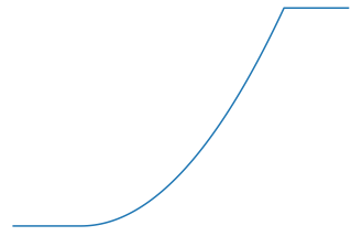
$\triangle Red$は$t=-\tau_\triangle$の時に$A_{ul}A_{ur}$を超え、$t=-\tau_\Box$の時、図形全体が収まる。また、その間の増加は下に凸の二次関数である。
S_{\triangle Red}(t) =
\begin{cases}
0 &
    (t<-\tau_\triangle)\\
\frac{1}{2}\frac{1}{\tau_\triangle-\tau_\Box}\left(t+\tau_\triangle\right)^2 &
    (-\tau_\triangle\leq t\leq-\tau_\Box)\\
\frac{\tau_\triangle-\tau_\Box}{2} &
    (-\tau_\Box<t)
\end{cases}
$\Box White$は$t=\min(-\tau_\Box,\tau_\Box)$の時に$A_{ul}A_{ur}$を超え、$t=\max(-\tau_\Box,\tau_\Box)$の時、図形全体が収まる。また、その間の増加は一次関数的であるため、
S_{\Box White}(t) =
\begin{cases}
0 &
    (t<-\tau_\Box)\\
t+ \tau_\Box &
    (-\tau_\Box\leq t)\\
\end{cases}
+
\begin{cases}
0 &
    (t<\tau_\Box)\\
-t+ \tau_\Box &
    (\tau_\Box\leq t))\\
\end{cases}
$\triangle Blue$は$t=\tau_\Box$の時に$A_{ul}A_{ur}$を超え、$t=\tau_\triangle)$の時、図形全体が収まる。また、その間の増加は上に凸の二次関数である。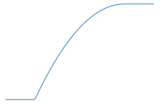
よって、これは$S_{\triangle Red}(t)$を原点対象に点対称移動させた後、$\frac{\tau_\triangle-\tau_\Box}{2}$を足した関数と等しい。
S_{\triangle Blue}(t) = \frac{\tau_\triangle-\tau_\Box}{2}-S_{\triangle Red}(-t)
コード
初期条件は以下の通り。
import numpy as np
import matplotlib.pyplot as plt

x, y  = np.mgrid[:10,:10]
a, b, c = 2, -1, -1
w = 1
tの計算
これは簡単。ピクセルと直線の距離に0.5を足すだけ。
import numpy as np
import matplotlib.pyplot as plt

x, y  = np.mgrid[:10,:10]
a, b, c = 2, -1, -1
w = 1

t = - b/a * y - c/a - x + 0.5
τの計算
$\theta$を介さずに計算する。
tau_triangle = (w*(a**2 + b**2)**0.5/a - b/a)/2
tau_square = (w*(a**2 + b**2)**0.5/a + b/a)/2
S_Xの計算
# S_blueでも使うため、S_redを関数で宣言
S_red_func = lambda t :\
        np.where(t<-tau_triangle,0,
        np.where(t<= -tau_square,(t+tau_triangle)**2/(2*(tau_triangle - tau_square)),
                                 (tau_triangle - tau_square)/2))
S_red = S_red_func(t)
S_blue = (tau_triangle - tau_square)/2 - S_red_func(-t)
S_white = np.where(t<-tau_square,0, t+tau_square) + \
          np.where(t<tau_square,0, -t+tau_square)

# S_Bを作成
S_B = S_red + S_blue + S_white
S_Xの差を計算
np.diffを用いる。$S_B(t)-S_B(t-1)$を計算するには、引き算の前後を整えるために-np.diff(S_B)
を使う。
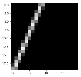
また、白地に黒の直線にするための変換も行う。
img_how_long_did_it_take_to_get_this = -np.diff(S_B,axis = 0)

# 最大値は1ピクセルの面積=1
img_black = 1-img_how_long_did_it_take_to_get_this
plt.imshow(img_black, cmap = 'gray')

ここで、diffをとっているため、縦方向のピクセルが1減っていることに留意してほしい。
関数としてまとめる
$a\geq-b\geq0,a>0$の条件を外したうえで、関数をつくる。(なお、a,bが0の時の例外処理はしていない)
def my_antialias(height, width, a, b, c, w=1):
    '''高さheight、幅widthの平面に太さwの直線ax + by + c = 0をアンチエイリアスで描画する。'''

    #diffをとったときに大きさが減る分を先に足しておく
    x, y  = np.mgrid[:height + 1,:width]

    #tを計算(a倍している)
    t = 0.5*a - (a*x + b*y + c)

    #τを計算(a倍している)
    tau_triangle = (w*(a**2 + b**2)**0.5 +abs(b))/2
    tau_square = (w*(a**2 + b**2)**0.5 - abs(b))/2

    #Sの計算
    S_red_func = lambda t :\
            np.where(t<-tau_triangle,0,
            np.where(t<= -tau_square,(t+tau_triangle)**2/(2*(tau_triangle - tau_square)),
                                     (tau_triangle - tau_square)/2))
    S_red = S_red_func(t)
    S_blue = (tau_triangle - tau_square)/2 - S_red_func(-t)
    S_white = np.where(t<-tau_square,0, t+tau_square) + \
              np.where(t<tau_square,0, -t+tau_square)

    #t,τがa倍されているのでaで割る
    S_B = (S_red + S_blue + S_white)*a
    return -np.diff(S_B,axis = 0)
plt.imshow(my_antialias(20,20,-3,-7,60,1),cmap = 'gray',vmin = 0,vmax=1)
plt.show()
ちなみに以下はブレゼンハムのアルゴリズム擬きで生成した直線である。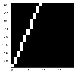
わたしの実行環境ではブレゼンハムのアルゴリズムを用いたほうが3~4倍速かった。