はじめに
機械学習コンペサイト"Kaggle"にて話題に上がるLightGBMであるが,Microsoftが関わるGradient Boostingライブラリの一つである.Gradient Boostingというと真っ先にXGBoostが思い浮かぶと思うが,LightGBMは間違いなくXGBoostの対抗位置をねらっているように見える.理論の詳細についてはドキュメントを参照いただくとして,本記事では「ハンズオン」ということで新しいツールの使い方を紹介したい.
まず,ドキュメント冒頭から引用させていただく.
LightGBM is a gradient boosting framework that uses tree based learning algorithms.
It is designed to be distributed and efficient with the following advantages:
- Faster training speed and higher efficiency
- Lower memory usage
- Better accuracy
- Parallel learning supported
- Capable of handling large-scale data
LightGBM の売り文句であるが,かい摘んで言うと「速くで正確!」ということ.XGBoostの特長とダブって聞こえるが,ライブラリの構成もとても似ている.
- ソースコードのコア部分は,C++.それをCLI(Command Line Inteface)で実行可能.
- Pythonプログラマには,Python-Packageがサポートされる.
- Rプログラマには,R-Package(本稿執筆時でbetaバージョン)がサポートされている.
今回は,Pythonにてコード確認をしてみた.(プログラミング環境は,Ubuntu 16.04LTS, Python 3.5.2, miniconda3, LightGBM 0.1 になります.)
(追記,2017/1/14, R-Packageについても試してみました.)
LightGBMの特徴 ー XGBoostとの違い
簡単にBoostingのコンセプトを下の図で確認する.
(「はじめてのパターン認識」の第11章からの引用(体裁を少し変更)になります.)
Fig. Boosting concept
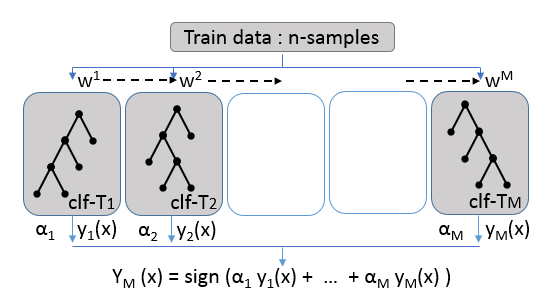
決定木の弱識別器を直列に複数並べ,これらに訓練データをサンプリングし重み($w^1$, $w^2$,.. $w^M$)をつけたものを入力する.各識別器の学習はシーケンシャルに行い,入力データの重みはこの学習結果を反映させる.アンサンブル識別器の予測値として,$Y_M$は,弱識別器の予測値を線形結合した値を得る.
次に,"LightGBM" の特徴をドキュメントにて確認しておく.
(参考)Optimization in speed and memory usage
"XGBoost"を含む多くのツールでは,決定木学習のに"pre-sorted"ベースで行うが,"LightGBM"では"histogram based algorithms"を用いるとのこと.この手法の特長としては,
- Reduce calculation cost of split gain
- Use histogram subtraction for further speed-up
- Reduce Memory usage
- Reduce communication cost for parallel learning
が挙げられるが,要は「軽く」て「効率がいい」ということらしい.
(アルゴリズムの違い詳細を理解するためには,論文をいくつか読み込む必要があります.参考文献リストのリンクは こちら になります. ネットで検索してみましたが,内容は難しそうです...)
また,学習の過程で,多くのツールがlevel(depth)-wiseで木を成長させていくのに対し,LightGBMではleaf-wiseで成長させるとのこと.
Fig. Leaf-wise tree growth
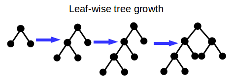
(ドキュメントに分かりやすい 説明図 がありますので,参照ください.)
このleaf-wiseのやり方に対応して,"overfit"に関するパラメータ設定で注意が必要となるが,これについては後で触れる.
以上,XGBoostとLightGBMは同じ決定木(Decision Tree)ベースのアンサンブルモデルであるが,アルゴリズム詳細に違いがあるということを確認した.
インストールと最初のコード
私の環境(Ubuntu 16.04 + miniconda)において,ソースコードのコンパイルはドキュメントの手順で問題なく完了した.その後,Python-Packageのインストール処理で少し手間取った.Python-Packageのインストールでは,以下を実施するが,
cd python-package; python setup.py install
ここで次のエラーが発生するケースがある.
error: Error: setup script specifies an absolute path:

/Users/Microsoft/LightGBM/python-package/lightgbm/../../lib_lightgbm.so

setup() arguments must always be /-separated paths relative to the setup.py directory, never absolute paths.
(この「絶対パスを使うな」のエラーについてはドキュメントでも触れられているが,現象/再現性がはっきりしていない.実際,私も2台のPC(Ubuntu)にLightGBMをインストールしてみたが,1台で上記エラーが発生し,もう1台ではエラーの発生はなかった.)
エラーの原因は,Pythonの"setuptools"バッケージ周りにありそうので,(あまり推奨される方法ではないのかもしれないが)以下のようにsetup.pyの一部を修正してエラー回避をすることができた.
修正箇所: 関数で`LIB_PATH`を生成しているところをマスクし,所定のパスをベタ書き.

 libpath = {'__file__': libpath_py}
 exec(compile(open(libpath_py, "rb").read(), libpath_py, 'exec'), libpath, libpath)

-LIB_PATH = libpath['find_lib_path']()
+# LIB_PATH = libpath['find_lib_path']()
+LIB_PATH = ['../lib_lightgbm.so']
 print("Install lib_lightgbm from: %s" % LIB_PATH)
さてコード作成にとりかかるが,ライブラリが若いからかリポジトリ内の例題コードが少ない.以下,少し試行錯誤しながら,各例題を扱ってみた.
分類問題(Classification)
まず,"iris"データセットの分類である.
import numpy as np
import lightgbm as lgb
from sklearn.datasets import load_iris
from sklearn.model_selection import train_test_split
from sklearn.metrics import accuracy_score


iris = load_iris()
X = iris.data
y = iris.target

X_train, X_test, y_train, y_test = train_test_split(
        X, y, test_size=0.2, random_state=0)

lgb_train = lgb.Dataset(X_train, y_train)
lgb_eval = lgb.Dataset(X_test, y_test, reference=lgb_train)

# LightGBM parameters
params = {
        'task': 'train',
        'boosting_type': 'gbdt',
        'objective': 'multiclass',
        'metric': {'multi_logloss'},
        'num_class': 3,
        'learning_rate': 0.1,
        'num_leaves': 23,
        'min_data_in_leaf': 1,
        'num_iteration': 100,
        'verbose': 0
}

# train
gbm = lgb.train(params,
            lgb_train,
            num_boost_round=50,
            valid_sets=lgb_eval,
            early_stopping_rounds=10)
y_pred = gbm.predict(X_test, num_iteration=gbm.best_iteration)
y_pred = np.argmax(y_pred, axis=1)
使い方は,"XGBoost" とかなり似ている.まず,lightgbm.Datasetオブジェクトを生成して,入力データをセットする.所定のパラメータを用意して,分類器(Classifier)モデルを作成し,Trainデータにfitさせて分類器モデルを得る.パラメータについては,"XGBoost"と類似するところもあるが,異なるところもあるのでそこは覚える必要がある.
関連情報(ドキュメント)へのリンク
一つ覚えておきたいのが,決定木の数量に関するパラメータで,これは前述した"level(depth)-wise"から"leaf-wise"に変わることを考慮しなければならない.以下パラメータ変換について,ドキュメントから引用する.
Convert parameters from XGBoost
LightGBM uses leaf-wise tree growth algorithm. But other popular tools, e.g. XGBoost, use depth-wise tree growth. So LightGBM use
num_leavesto control complexity of tree model, and other tools usually usemax_depth. Following table is the correspond between leaves and depths. The relation isnum_leaves = 2^(max_depth).
max_depth num_leaves 1 2 2 4 3 8 7 128 10 1024
このルールを覚えてしまえば,特に問題なさそうである.例えば"XGBoost"の max_depth=6 の設定と同等にするには,num_leaves=64 と設定すればよい.
回帰問題(Regression)
次に回帰(Regression)を試してみる.扱ったデータセットは,"boston" (housing data set)である.(最近のScikit-learnには "boston"も付属しており,load_boston() でデータを入力することができる.)
import numpy as np
import lightgbm as lgb
from sklearn.datasets import load_boston
from sklearn.metrics import mean_squared_error
from sklearn.model_selection import KFold, train_test_split

print("Boston Housing: regression")
boston = load_boston()
y = boston['target']
X = boston['data']

X_train, X_test, y_train, y_test = train_test_split(
    X, y, test_size=0.33, random_state=201612
)

# create dataset for lightgbm
lgb_train = lgb.Dataset(X_train, y_train)
lgb_eval = lgb.Dataset(X_test, y_test, reference=lgb_train)
# LightGBM parameters
params = {
        'task' : 'train',
        'boosting_type' : 'gbdt',
        'objective' : 'regression',
        'metric' : {'l2'},
        'num_leaves' : 31,
        'learning_rate' : 0.1,
        'feature_fraction' : 0.9,
        'bagging_fraction' : 0.8,
        'bagging_freq': 5,
        'verbose' : 0
}

# train
gbm = lgb.train(params,
            lgb_train,
            num_boost_round=100,
            valid_sets=lgb_eval,
            early_stopping_rounds=10)
y_pred = gbm.predict(X_test, num_iteration=gbm.best_iteration)
大部分,分類問題(Classification)と同じだが,LightGBMモデルに渡すパラメータで,'objective' を 'regression'に(分類(多クラス分類)では 'multiclass'),'metric' を 'l2' (分類では 'multi_logloss') に変更する必要がある.
Scikit-learnインターフェース
これも先行ツール同様に,Scikit-learn のインターフェースが用意されている.ネイティブに近いインターフェースの方が,細かい操作ができたり,新しい機能のサポートが早かったりするケースもあるが,個人的にはScikit-learnインターフェースの方を使っていきたい.(次々と新規ライブラリが登場している中で,できるだけ覚える事を少なくしたい,というのが第一の理由である.)
gbm = lgb.LGBMClassifier(objective='multiclass',
                        num_leaves = 31,
                        learning_rate=0.1,
                        min_child_samples=10,
                        n_estimators=100)
gbm.fit(X_train, y_train,
        eval_set=[(X_test, y_test)],
        eval_metric='multi_logloss',
        early_stopping_rounds=10)
y_pred = gbm.predict(X_test, num_iteration=gbm.best_iteration)
おなじみのインターフェース,分類器のインスタンスを生成して,その後,fit() するという流れである.
early stopping も上記コードで問題なく動いている.
主に使うクラスは,次の2つになる.
- LGBMClassifier
- LGBMRegressor
アンサンブルのベースモデルとして
前述の通り,Gradient Boosting自体,決定木識別器のアンサンブル手法であるが,ここでは,"LightGBM", "XGBoost"をベースモデルとして用いた,メタモデリングという意味でのアンサンブルを取り上げる.
アンサンブルをする際に「Bias-Variance について異なる出力をする複数のモデルを用いるとよい」というアドバイスがあるが,異なる結果をもらたらすモデル自体の予測性能がある程度確保されていないと,アンサンブルをやっても全体の精度が上がらなくて悩むことが多い.例えば,Logistic Regressionと(チューニングされていない)Neural NetworkモデルとXGBoost モデルを,時間をかけてアンサンブルしたにも関わらず,その精度が(一番高性能な)XGBoost単体の結果と変わらないという状況を経験したことがある.「粒が揃ったベースモデル」を用意する目的で,"LightGBM" を "XGboost" と併用するオプションが思いつく.(kaggleでもそんなコード,フォーラム意見がありました.)以下,それぞれのベースモデルを実装したコード例を挙げる.
LightGBM のベースモデル
def lgb_analysis(X_train, X_test, y_train, y_test, n_folds=5):
    '''
      Base analysis process by LightGBM
    '''
    kf = KFold(n_splits=n_folds, random_state=1)
    y_preds_train = []
    y_preds_test = []
    for k, (train, test) in enumerate(kf.split(X_train, y_train)):
        gbm = lgb.LGBMClassifier(objective='multiclass',
                        num_leaves = 23,
                        learning_rate=0.1,
                        n_estimators=100)
        gbm.fit(X_train[train], y_train[train],
            eval_set=[(X_train[test], y_train[test])],
            eval_metric='multi_logloss',
            verbose=False,
            early_stopping_rounds=10)
        y_pred_train = gbm.predict_proba(X_train[test],
                            num_iteration=gbm.best_iteration)
        y_pred_test = gbm.predict_proba(X_test,
                            num_iteration=gbm.best_iteration)
        y_pred_k = np.argmax(y_pred_test, axis=1)
        accu = accuracy_score(y_test, y_pred_k)
        print('fold[{:>3d}]: accuracy = {:>.4f}'.format(k, accu))
        y_preds_train.append(y_pred_train)
        y_preds_test.append(y_pred_test)

    return y_preds_train, y_preds_test
XGBoost のベースモデル
def xgb_analysis(X_train, X_test, y_train, y_test, n_folds=5):
    '''
      Base analysis process by XGBoost
    '''
    kf = KFold(n_splits=n_folds, random_state=1)
    y_preds_train = []
    y_preds_test = []
    for k, (train, test) in enumerate(kf.split(X_train, y_train)):
        xgbclf = xgb.XGBClassifier(objective='multi:softmax',
                        max_depth=5,
                        learning_rate=0.1,
                        n_estimators=100)
        xgbclf.fit(X_train[train], y_train[train],
            eval_set=[(X_train[test], y_train[test])],
            eval_metric='mlogloss',
            verbose=False,
            early_stopping_rounds=10)
        y_pred_train = xgbclf.predict_proba(X_train[test])
        y_pred_test = xgbclf.predict_proba(X_test)
        y_pred_k = np.argmax(y_pred_test, axis=1)
        accu = accuracy_score(y_test, y_pred_k)
        print('fold[{:>3d}]: accuracy = {:>.4f}'.format(k, accu))
        y_preds_train.append(y_pred_train)
        y_preds_test.append(y_pred_test)

    return y_preds_train, y_preds_test
これらの関数を使ってアンサンブルし,scikit-learnの"digit dataset"を分類した実行状況が以下である.
LightGBM process:
[LightGBM] [Warning] Ignoring Column_0 , only has one value
[LightGBM] [Warning] Ignoring Column_32 , only has one value
[LightGBM] [Warning] Ignoring Column_39 , only has one value
fold[  0]: accuracy = 0.9360
[LightGBM] [Warning] Ignoring Column_0 , only has one value
[LightGBM] [Warning] Ignoring Column_32 , only has one value
[LightGBM] [Warning] Ignoring Column_39 , only has one value
fold[  1]: accuracy = 0.9394
[LightGBM] [Warning] Ignoring Column_0 , only has one value
[LightGBM] [Warning] Ignoring Column_32 , only has one value
[LightGBM] [Warning] Ignoring Column_39 , only has one value
fold[  2]: accuracy = 0.9394
[LightGBM] [Warning] Ignoring Column_0 , only has one value
[LightGBM] [Warning] Ignoring Column_32 , only has one value
[LightGBM] [Warning] Ignoring Column_39 , only has one value
[LightGBM] [Warning] Ignoring Column_56 , only has one value
fold[  3]: accuracy = 0.9276
[LightGBM] [Warning] Ignoring Column_0 , only has one value
[LightGBM] [Warning] Ignoring Column_24 , only has one value
[LightGBM] [Warning] Ignoring Column_32 , only has one value
[LightGBM] [Warning] Ignoring Column_39 , only has one value
fold[  4]: accuracy = 0.9310
XGBoost process:
fold[  0]: accuracy = 0.9377
fold[  1]: accuracy = 0.9411
fold[  2]: accuracy = 0.9444
fold[  3]: accuracy = 0.9343
fold[  4]: accuracy = 0.9310

Stacked model:
accuracy = 0.9512

confusion matrix:
[[49  0  0  0  0  0  0  0  0  0]
 [ 1 57  1  0  1  0  0  0  0  1]
 [ 2  0 57  0  0  0  1  0  2  0]
 [ 0  0  0 54  0  0  0  0  0  1]
 [ 0  0  0  0 49  0  0  1  0  0]
 [ 0  0  0  1  0 61  1  0  0  2]
 [ 0  0  1  0  0  0 66  0  0  0]
 [ 0  0  0  0  1  0  0 55  0  0]
 [ 0  4  0  2  0  0  0  0 60  1]
 [ 1  0  0  2  0  2  0  0  0 57]]
アンサンブルで若干の精度(正答率)upを実現できている.(Warningが発生していますが.)
いかがだろうか? ここではアンサンブル(stacking)についての説明は省くが,上の2つのコードで雰囲気は感じていただけるかと思う."LightGBM", "XGBoost" 共にScikit-learn APIを用いることにより,大部分同じでいくつかのキーワードを変えるだけで,2つのモデルを実装できた.
また,欲しい性能についても,細かいアルゴリズムの違い("histogram based algorithms"や "leaf-wise growth"の特徴)により,「似て非なる」ベースモデルの結果が期待できるのではないだろうか? (まだ,性能確認中ですが...)
以上,簡単に "LightGBM" について紹介させていただいた.まだ ver.0.1 であるが,かなり完成度が高い印象をもった.RプログラマにもR-Packageがあるので,この"LightGBM"を推奨したい.
(追記)R-Packageについても試した
R-Packageも先日,サポートされたので試してみた.まず,R-Packageの入れ方は,次の通り.
方法1:(ソースコードのコンパイル後,)
cd R-package
R CMD INSTALL --build  .
方法2:({devtools}でリポジトリから直接インストール)
devtools::install_github("Microsoft/LightGBM", subdir = "R-package")
こちらも "iris" の分類を行った.
library(lightgbm)
data(iris)

# split data to train / test
set.seed(2017)
train_size = 100    # test_size is 50
train_ind <- sample(seq_len(nrow(iris)), size = train_size)

train <- iris[train_ind, ]
test <- iris[-train_ind, ]
x_train <- train[, -5]
y_train <- as.numeric(train[, 5]) - 1   # need zero start labelling, [0, 1, 2]
x_test <- test[, -5]
y_test <- as.numeric(test[, 5]) - 1     # need zero start labelling, [0, 1, 2]

# model definition and training
bst <- lightgbm(data = as.matrix(x_train), label = y_train,
        num_leaves = 4, learning_rate = 0.1, nrounds = 20,
        min_data = 20, min_hess = 20,
        objective = "multiclass", metric="multi_error",
        num_class = 3, verbose = 0)

# make prediction
y_pred_proba <- matrix(predict(bst, as.matrix(x_test)), byrow=T, ncol=3)
y_pred <- apply(y_pred_proba, 1, which.max) - 1

# confusion matrix
cat("\n confusion matrix:\n")
table(y_test, y_pred)
少しはまったのが,”iris" の数値化したクラスラベルが [1, 2, 3] では”LightGBM"の関数が受け付けず,[0, 1, 2] にシフトする必要があった点である.(初見のエラーでしたので,少し戸惑いました.)
参考文献,web site
- Miscrosoft/LightGBM - GitHub
https://github.com/Microsoft/LightGBM - LightGBMのPythonパッケージ触ってみた - marugari2さんブログ
http://marugari2.hatenablog.jp/entry/2016/12/14/235747 - はじめてのパターン認識,平井氏著,森北出版
https://www.morikita.co.jp/books/book/2235