誰向け
深層学習をすでに理解して画像の分類から物体検出への仕組みをマスターしたい方へ
数式が多いのでコード確認したい方は下記へGo
おまけ
Kerasに関する書籍を翻訳しました。画像識別、画像生成、自然言語処理、時系列予測、強化学習まで幅広くカバーしています。
直感 Deep Learning ―Python×Kerasでアイデアを形にするレシピ
目的
物体検出に関しての技術を体系的にまとめてコードベースまで理解したかったので書きました。
良書である画像認識の物体認識の章を参考にこの記事を作成しています。
全体像
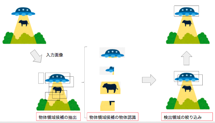
大きく分けて3つのフェーズに分かれます。
1: 物体領域候補の抽出
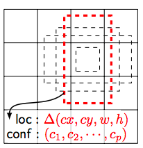
画像中から物体の領域候補を抽出する手法になります。精度と速度を左右する部分になります。図のように小ウインドウ(バウンディングボックス)を用意して一定の画素数ずらしながら領域候補を抽出する手法があります。これは1画素ごとにずらすと画像のサイズW*Hの評価が必要になります。そこでこの計算コストを減らすために物体の画像らしさを評価する手法で候補を絞り込むことが一般的です。
2: 物体領域候補の物体認識
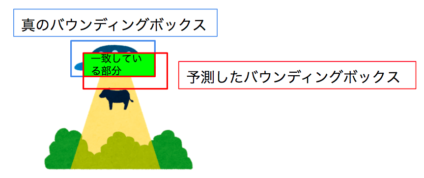
候補に何が写っているかを認識する必要があります。ここは一般的な教師ありの分類問題で解くことが可能です。ここで重要になってくるのが教師データの選定です。負例(間違っているデータ)は分類が困難な例を選ばないと簡単な問題しか解けない分類器となり実用に耐えない性能になります。そこで分類困難な負例として選ぶことが重要になります。この図だと牛の全体像が取れている部分は負例として適切です。
3: 検出領域の絞り込み
対象となる物体が一つであっても複数領域が出てきます。この中から検出スコアが最大値のみの部分を選定することで適切な検出領域を決定します。
各手法
| 物体領域候補の抽出 | 物体領域候補の物体認識 | 検出領域の絞り込み |
|---|---|---|
| スライディングウィンドウ方式(非効率だが単純) | HOG特徴 + 線形SVM | NMS(IoUが用いられる) |
| 選択的検索法(効率的) | DPM(物体の変形を考慮) | |
| 分岐限定法(効率的) | ホグ特徴 + LatentSVM(フィルター位置考慮) | |
| attentional cascade(高速な物体検出ただし分類器が必要) | Exampler-SVM(個々の物体に対して分類を行う) | |
| 矩形特徴 + Adaboost(低コストながら分類性能高い) |
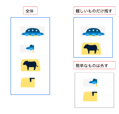
物体領域候補の物体認識における良い負例の集め方は分類器が誤って分類した負例をキャッシュとしてためておき、分類できた負例の候補は外していくことによって効率よく集めて学習することができます。
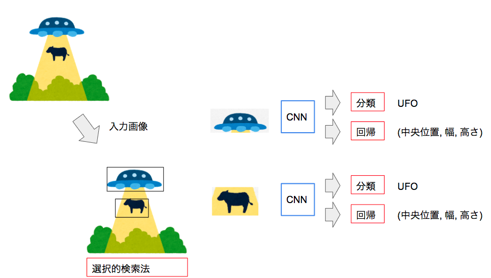
深層学習による物体検出
深層学習による物体検出は上記の手法に比べて良質な特徴が抽出可能なCNN特徴が使える点が利点になります。では実際に深層学習による物体検出のフローを見てみましょう。
ここからは小ウインドウのことをバウンディングボックスと表します。
R-CNN (Region)
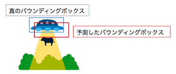
バウンディングボックスの回帰の手法ですが提案したバウンディングボックスを
\vec{r} = (r_x, r_y, r_w, r_h)^T
真のバウンディングボックス
\vec{g} = (g_x, g_y, g_w, g_h)^T
真のバウンディングボックスを得るためのモデルのパラメータWは下記で解きます。
\vec{W} = argmin_{\vec{w}}\sum^{N}_{n=1}({\vec{t}_n - \vec{W}^Tf(\vec{r}_n)})^2 + \lambda\|\vec{W}\|^2_{F}
ここで目標となる回帰のための値
\vec{t} = (t_x, t_y, t_w, t_h)^T
tは先ほど定義した真のバウンディングボックスgと提案したバウンディングボックスrを使用する
t_x = (g_x - r_x) / r_w,
t_y = (g_y - r_y) / r_h,
t_w = log(g_w / r_w),
t_h = log(g_h / r_h),
上記のように定義します。上記のようにしている理由は下記のように推測されます。推測の理由は書籍になかったのと調査してないからです。気になる方は調べていただけると助かります。
バウンディングボックスのサイズは様々な種類であるため中央位置は差分の値から幅の値の比率によって算出する。
幅の値は真の値との比率で算出。ただし値が極端に小さくなったり大きくなる可能性があるため対数によってその影響を減らす。
上記のために直接的に値を使用せずに工夫していると思われます。
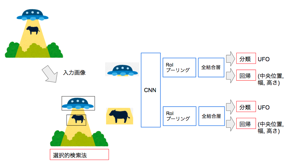
Fast R-CNN
R-CNNは物体領域ごとにCNNをする必要がありました。Fast R-CNNはCNN特徴は画像全体を使う点が異なります。その際に切り取った画像領域ごとにCNN特徴量が異なるのでRoIプーリングによって固定長の特徴量に変換する必要がある点が異なります。
RoIプーリングとは下記の10ページを参照
学習方法
クラス認識とバウンディングボックスへの回帰を同時学習するためマルチタスク損失を最適化する方法を取ります。
各正解バウンディングボックスにR-CNNで求めた時に使用した正解位置tとラベルuが付与されているとします。マルチタスク損失は下記の式で表します。
クラスの事後確率
\vec{p} = (p^0, p^1,... p^N_c)^T
バウンディングボックスの相対的な位置と大きさ
\vec{v} = (v_x, v_y, v_w, v_h)^T
上記を踏まえて
J(\vec{p}, u, \vec{v}, \vec{t}) = J_{cls}(\vec{p}, u) + \lambda[u >= 1]J_{loc}(\vec{v}, \vec{t})
J_clsはクラス認識の損失でJ_locはバウンディングボックスの回帰の損失です。
J_clsは真のクラスuに対する事後確率p^uの負の対数で計算します。
J_{cls}(\vec{p}, u) = -\log{p^u}
J_locは
J_{loc} = \sum_{i \in { \{x,y,w,h} \}}smooth_{L1}(t_i - v_i)
smooth_{L1}(x) = \left\{
\begin{array}{ll}
0.5x^2 & if (|x| < 1) \\
|x| - 0.5 &otherwise
\end{array}
\right.
smooth関数によって相対的な位置の差が1より小さい時は大きくなるようにそれ以外の時は0.5の中央値で引いて極端に大きな値にならないように補正しています。
計算の効率化
全結合が画像ごとに処理されるため一つの画像でミニバッチが動作するようにして効率よく特徴マップを使用できるようにします。具体的にはN(画像枚数)を小さいくしてR(バウンディングボックスの数)を大きくします。
Faster R-CNN
Fast R-CNNでは物体領域候補を別モジュール(選択的検出法)で計算する必要がありました。Faster R-CNNではRPNという特徴量マップから物体領域を推定する領域ネットワークを作りFast R-CNNと統合するやり方を取っています。
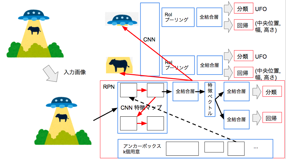
RPNによってスコア付きのバウンディングボックスを提案します。
RPNではバウデンィングボックスのパラメータを学習する部分と物体の有無を予測する分離ネットワークで構成されておりこれを結合してRPNを実現しています。
あらかじめ形状が決められたK個のアンカーボックスを用意しておきます。入力の局所領域(これはエッジの算出などで導出)を中心とした標準的なバウンディングボックスを用意しておきます。この辺はハイパーパラメータ的な要素。
バウンディングボックスの予測は各アンカーボックスからの相対的な位置とアスペクト比を含んだ4k次元のベクトルを出力します。(x, y, w, h) * k
分類ネットワークは物体の有無を2クラスで判断するので2k次元のベクトルを出力します。(有り,無し) * k
Fast R-CNNと同様のマルチタスク損失を最小化することによって最適なバウンディングボックスを導出します。
RPNとFast R-CNNを交互に学習することでFaster R-CNNのネットワーク全体を学習します。まずRPNのみで学習して最適なバウンディングボックスを導出できるようにしてからR-CNNを学習して、そのあとにFast R-CNNを学習します。
YOLO (You only look once)
ここまでは良いバウンディングボックスを求めることが主題でしたが直接的に物体検出をしようという試みが有ります。それがYOLOです。
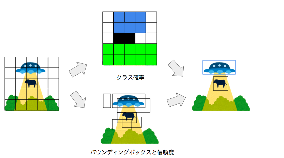
YOLOの手順
1: 入力画像をS*Sの領域に分割
2: 領域内の物体のクラス確率を導出
3: B個(ハイパーパラメータ)のバウンディングボックスのパラメータ(x, y, h, w)と信頼度を計算
信頼度
q = P_r(Obj) \times IoU^{truth}_{pred}
IoU^{truth}_{pred}
は予測と正解のバウンディングボックスの一致度です。
物体検出には物体クラス確率と各バウンディングボックスの信頼度の積を用います。
P_r(C_i|Obj) \times P_r(Obj) \times IoU^{truth}_{pred}
YOLOのネットワークは下記になります。
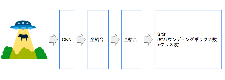
出力はS*Sに分割した画像領域と(x,y,h,w)と信頼度を含むバウンディングボックスの数とクラス数になります。
信頼度は下記の式で表します。バウンディングボックスの一致度を測ります。
IoU = \frac{area(R_p \bigcap R_g)}{area(R_p \bigcup R_g)}
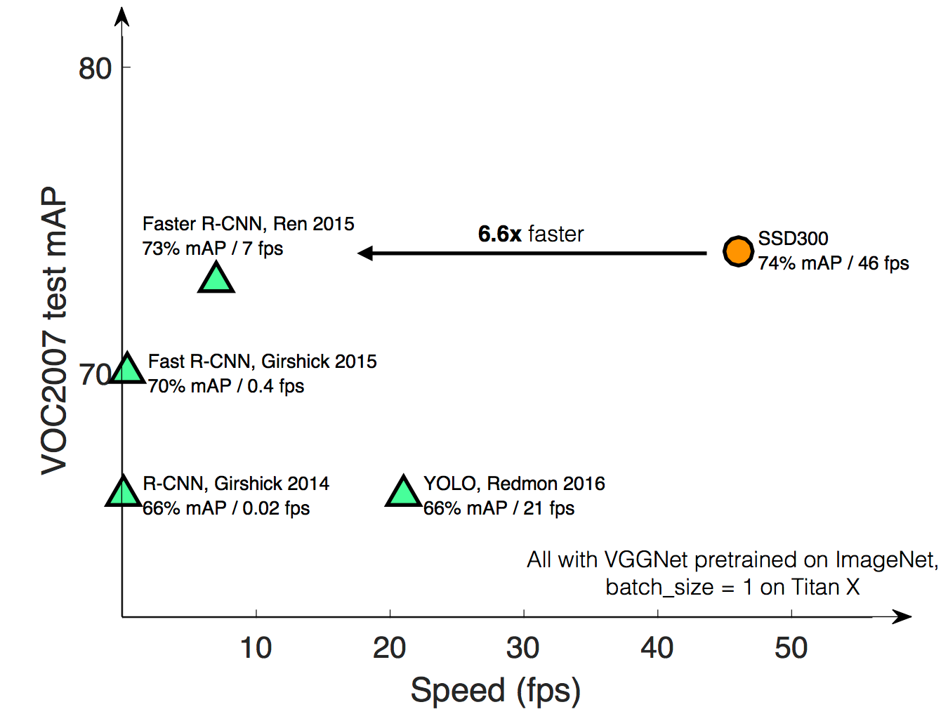
SSD
書籍には有りませんでしたが手法として有用なSSDについてもふれておきます。
・速度比較
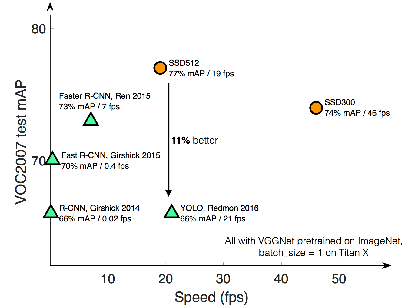
・精度比較
SSD512とSSD300の違いは入力画像のサイズ
利点
- YOLOと同様にシンプルなネットワーク構成
- 高速
- 精度が高い
利点の理由
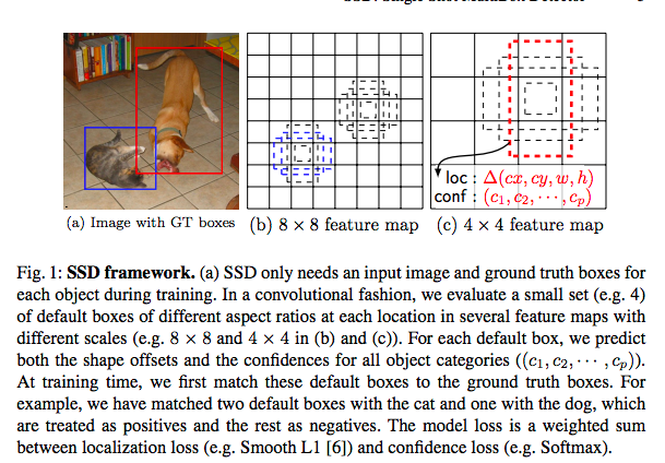
- アスペクト比に応じた出力層を用意して学習させることによって画像のスケールに影響されないモデルの提供
- End to Endのシンプルなモデルにより余分な処理が不要な分、高速
modelの比較
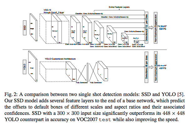
End to EndのモデルのYOLOとSSDを比較したのが上図です。
SSDの場合はアスペクト比の異なる特徴マップを複数用意してそれを最終層に入力することで画像の解像度が異なる場合でも適用できるようにしています。
出力層について
図中の8732の意味はボウンディングボックスの数です。数が多ければ精度が上がりますが速度が下がるのでトレードオフの関係になります。
出力層はクラス数Cとオフセット(x, y, h, w)、それらに紐づいたバウンディングボックスの数kそれらを各特徴マップごとに用意する必要があるので特徴マップのサイズがm*nの場合は下記が出力層のサイズになります。
(c+4)kmn
損失関数は物体の位置のズレとクラスの分類のズレの2点を求めることになります。Nはマッチしたデフォルトのバウンディングボックスの数(0の場合は損失が無限大に発散するため0を設定)。αはハイパーパラメータクラス識別かオフセットの回帰の重要性を制御)
ここでxは真のデータjのボックスと予測データのボックスiが一致すれば1、一致しない場合は0(pはクラス)
x^p_{ij} = {1, 0}
L(x,c,l,g) = 1/N(L_{conf}(x, c) + \alpha L_{loc}(x,l,g))
位置に関する損失関数
lは予測した位置
L_{loc}(x,l,g) = \sum^N_{i \in Pos}\sum_{m \in {cx, cy, w, h}} x^k_{ij} {\rm smooth_{L1}}(l^m_i-\hat{g}^m_j)
smooth_{L1}(x) = \left\{
\begin{array}{ll}
0.5x^2 & if (|x| < 1) \\
|x| - 0.5 &otherwise
\end{array}
\right.
デフォルトのバウンディングボックスはd、真のバウンディングボックスはgで表し、真の値をバウンディングボックスのスケールに正規化すると
\hat{g}^{cx}_j = (g^{cx}_j - d^{cx}_i) / d^{w}_i,
\hat{g}^{cy}_j = (g^{cy}_j - d^{cy}_i) / d^{h}_i,
\hat{g}^{w}_j = \log(g^{w}_j / d^{w}_i),
\hat{g}^{h}_j = \log(g^{h}_j / d^{h}_i),
クラスに関する損失関数
最初の項は各クラスの予測を2つ目の項は背景の予測を表している
L_{conf}(x, c) = -\sum^N_{i \in Pos}x^p_{ij}\log(\hat{c}^p_i) -\sum^N_{i \in Neg}x^p_{ij}\log(\hat{c}^0_i)
クラス分類はソフトマックス関数
\hat{c}^p_i = \frac{\exp(c^p_i)}{\sum_p{\exp(c^p_i)}}
Choosing scales and aspect ratios for default boxes
特徴マップがマルチスケールのため、各特徴マップごとにどの大きさのオブジェクトを検出するか役割を与えます。mが大きくなるほどスケールが小さくなります。これはモデルが深い層ほど小さいなオブジェクトの検出を行なっている特徴マップになっていることを表しています。
s_k = s_{min} + \frac{s_{max} - s_{min}}{m-1}(k-1)
デファルトで用意するバウンディングボックスのアスペクト比を下記のようにして
a_r = {1, 2, 3, 1/2, 1/3}
それぞれの幅、高さを計算して、バウンディングボックスを用意します。
幅
w^a_k = s_k \sqrt{a_r}
高さ
h^a_k = s_k / \sqrt{a_r}
アスペクト比が1の場合は下記のスケールを適用したバウンディングボックスを用意します。
s_k' = \sqrt{s_ks_k+1}
Hard negative mining
負例のバウンディングボックスが多数出るので信頼度順にソートして上位からピックアップし3:1(負例:正例)の比率になるように修正
Data augmentation
- 画像全体
- 切り取った画像ごとの真の値との重なり度(Jaccard)が0.1, 0.3, 0.5, 0.7, 0.9でサンプルを選択
- 切り取った画像をランダムにサンプル
具体的な実装例
抽象的な概念ややり方は分かったと実装するにはどうするんだという声が聞こえてきそうです。
下記のコードを参考にKeras v2.0で実装を行います。
A port of SSD: Single Shot MultiBox Detector to Keras framework.
オリジナルのコードはkeras2.0系に対応していないのでプルリクで修正してくれているコードを参考にします。
Dockerによる環境提供を記述しました。
Modelの理解
TensorflowにはTensorboardという可視化ツールがあるのでそれを利用して可視化を行います。
- モデルの可視化
Tensorboardのモデルのグラフ化を行い、全体像を把握します。
CNNレイヤー
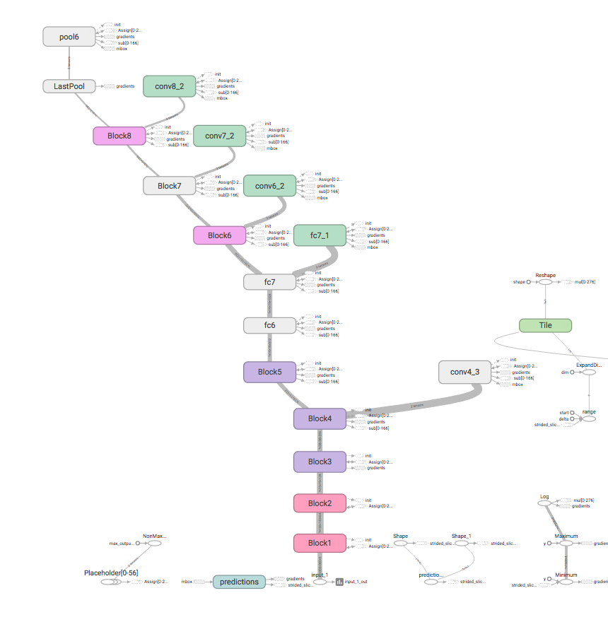
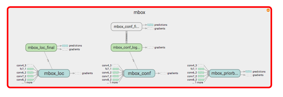
特徴マップを合体している部分
- オフセット(位置):
mbox_loc - 確信度 :
mbox_conf - 各バウンダリーボックス :
mbox_priorbox
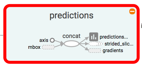
最終層
合体された特徴マップを用いて予測
具体的なコードの理解
概念図を理解した段階で具体的な処理を理解します。
モデルの記述
ssd_v2.py
ssdでは特徴マップの異なるレイヤーを合体して出力しています。
下記がオフセットとクラス識別の層をそれぞれコンカチしている処理です。0次元目がデータの次元なので1次元目の特徴量の次元が増える形になります。
        mbox_loc = concatenate([conv4_3_norm_mbox_loc_flat,
                                fc7_mbox_loc_flat,
                                conv6_2_mbox_loc_flat,
                                conv7_2_mbox_loc_flat,
                                conv8_2_mbox_loc_flat,
                                pool6_mbox_loc_flat],
                               axis=1, name='mbox_loc')
        mbox_conf = concatenate([conv4_3_norm_mbox_conf_flat,
                                 fc7_mbox_conf_flat,
                                 conv6_2_mbox_conf_flat,
                                 conv7_2_mbox_conf_flat,
                                 conv8_2_mbox_conf_flat,
                                 pool6_mbox_conf_flat],
                                axis=1, name='mbox_conf')
num_boxes = mbox_loc._keras_shape[-1] // 4
ボックスの数は位置の特徴量(全てがコンカチされたもの)を4で割ると得られるのでその値を利用します。
下記でコンカチした次元をオフセットの次元とクラスの識別の次元に修正しています。
num_boxesの次元:7308
mbox_locの次元:29232 (7308 * 4)
mbox_confの次元:153468 (7308 * クラス数(21))
        mbox_loc = Reshape((num_boxes, 4),
                           name='mbox_loc_final')(mbox_loc)
        mbox_conf = Reshape((num_boxes, num_classes),
                            name='mbox_conf_logits')(mbox_conf)
出力層ではオフセット、クラス識別、バウンディングボックス(x,y,h,wと各4座標のバリアンス)をコンカチしている処理です。
0次元目がデータの次元、1次元がバウンディングボックスの数の次元なので2次元目の特徴量の次元が増える形になります。
    predictions = concatenate([mbox_loc,
                               mbox_conf,
                               mbox_priorbox],
                              axis=2,
                              name='predictions')
SSDで必要な処理の記述
ssd_utils.pyはバウンディングボックスの設定を行なっています。
メソッド一覧
- decode_boxes:位置の予測を一致するバウンディングボックスの値に変換しています。
引数として位置の4つのオフセット、バウンディングボックスのオフセット、バウンディングボックスの分散を使用しています。
分散を利用する理由は一意に値が決まる訳ではないのである程度範囲を持った予測をできるようにするためです。
1: バウンディングボックスのオフセット情報から中心位置と幅、高さを求める
2: デコードするバウンダリーボックスを求めるため、先ほどの値と分散を利用してデコードしたバウンダリーボックスの中心位置と幅、高さを求める。予測した値は小さいのでexpにより十分な大きさの値に変換する。注意点として分散を考慮している点。予測した中央点と幅、高さは確率的なものを考慮して分散による値のズレを許容するため入れている。
3: 中心位置から最小、最大のオフセットのために変換する
4: 求めた値を一つのベクトルにまとめる
5: 変換した値から0以上かつ1以下の領域のみ返すようにする
    def decode_boxes(self, mbox_loc, mbox_priorbox, variances):
        prior_width = mbox_priorbox[:, 2] - mbox_priorbox[:, 0]
        prior_height = mbox_priorbox[:, 3] - mbox_priorbox[:, 1]
        prior_center_x = 0.5 * (mbox_priorbox[:, 2] + mbox_priorbox[:, 0])
        prior_center_y = 0.5 * (mbox_priorbox[:, 3] + mbox_priorbox[:, 1])

        decode_bbox_center_x = mbox_loc[:, 0] * prior_width * variances[:, 0]
        decode_bbox_center_x += prior_center_x
        decode_bbox_center_y = mbox_loc[:, 1] * prior_width * variances[:, 1]
        decode_bbox_center_y += prior_center_y
        decode_bbox_width = np.exp(mbox_loc[:, 2] * variances[:, 2])
        decode_bbox_width *= prior_width
        decode_bbox_height = np.exp(mbox_loc[:, 3] * variances[:, 3])
        decode_bbox_height *= prior_height

        decode_bbox_xmin = decode_bbox_center_x - 0.5 * decode_bbox_width
        decode_bbox_ymin = decode_bbox_center_y - 0.5 * decode_bbox_height
        decode_bbox_xmax = decode_bbox_center_x + 0.5 * decode_bbox_width
        decode_bbox_ymax = decode_bbox_center_y + 0.5 * decode_bbox_height

        decode_bbox = np.concatenate((decode_bbox_xmin[:, None],
                                      decode_bbox_ymin[:, None],
                                      decode_bbox_xmax[:, None],
                                      decode_bbox_ymax[:, None]), axis=-1)

        decode_bbox = np.minimum(np.maximum(decode_bbox, 0.0), 1.0)

        return decode_bbox
detection_out:予測した結果を返す
1: 予測した値から位置、分散、バウンディングボックス、確信度を取得
2: 位置の値をバウンディングボックスに変換
3: クラスの確信度が一定以上の場合はバウンディングボックスの値までを求める。
4: 上位200件の結果を返す
    def detection_out(self, predictions, background_label_id=0, keep_top_k=200,
                      confidence_threshold=0.01):

        mbox_loc = predictions[:, :, :4]
        variances = predictions[:, :, -4:]
        mbox_priorbox = predictions[:, :, -8:-4]
        mbox_conf = predictions[:, :, 4:-8]
        results = []
        for i in range(len(mbox_loc)):
            results.append([])

            decode_bbox = self.decode_boxes(mbox_loc[i],
                                            mbox_priorbox[i], variances[i])

            for c in range(self.num_classes):
                if c == background_label_id:
                    continue
                c_confs = mbox_conf[i, :, c]
                c_confs_m = c_confs > confidence_threshold
                if len(c_confs[c_confs_m]) > 0:
                    boxes_to_process = decode_bbox[c_confs_m]
                    confs_to_process = c_confs[c_confs_m]
                    feed_dict = {self.boxes: boxes_to_process,
                                 self.scores: confs_to_process}
                    idx = self.sess.run(self.nms, feed_dict=feed_dict)
                    good_boxes = boxes_to_process[idx]
                    confs = confs_to_process[idx][:, None]
                    labels = c * np.ones((len(idx), 1))
                    c_pred = np.concatenate((labels, confs, good_boxes),
                                            axis=1)
                    results[-1].extend(c_pred)

            if len(results[-1]) > 0:
                results[-1] = np.array(results[-1])
                argsort = np.argsort(results[-1][:, 1])[::-1]
                results[-1] = results[-1][argsort]
                results[-1] = results[-1][:keep_top_k]
        return results
ssd_layers.pyはバウンディングボックスのサイズを決めているPriorBoxのクラスを設定しています。図の黒線と赤線の部分です。
1: 特徴マップの幅と高さを取得
2: 入力画像の幅と高さを取得
3: アスペクト比に合わせてバウンディングボックスのサイズを追加
4: アスペクト比が1とそうでない時で処理が異なる。
5: ボックスの中央位置の定義
6: 最小位置と最大位置のバウンディングボックスの設定
7: 分散の設定
8: バウンディングボックスと分散を設定し、Tensorflowのフォーマットで返す
class PriorBox(Layer):

    # 省略

    def call(self, x, mask=None):
        if hasattr(x, '_keras_shape'):
            input_shape = x._keras_shape
        elif hasattr(K, 'int_shape'):
            input_shape = K.int_shape(x)

        layer_width = input_shape[self.waxis]
        layer_height = input_shape[self.haxis]

        img_width = self.img_size[0]
        img_height = self.img_size[1]
        # define prior boxes shapes
        box_widths = []
        box_heights = []

        for ar in self.aspect_ratios:
            if ar == 1 and len(box_widths) == 0:
                box_widths.append(self.min_size)
                box_heights.append(self.min_size)
            elif ar == 1 and len(box_widths) > 0:
                box_widths.append(np.sqrt(self.min_size * self.max_size))
                box_heights.append(np.sqrt(self.min_size * self.max_size))
            elif ar != 1:
                box_widths.append(self.min_size * np.sqrt(ar))
                box_heights.append(self.min_size / np.sqrt(ar))
        box_widths = 0.5 * np.array(box_widths)
        box_heights = 0.5 * np.array(box_heights)

        # 画像のサイズを特徴量のサイズで割ってステップ幅を取得
        step_x = img_width / layer_width
        step_y = img_height / layer_height
        # linspaceの処理
        #     https://docs.scipy.org/doc/numpy/reference/generated/numpy.linspace.html
        # np.linspace(2.0, 3.0, num=5)
        #   -> array([ 2.  ,  2.25,  2.5 ,  2.75,  3.  ])
        # ステップ幅ごとに特徴量の数分、縦、横のarrayを取得
        linx = np.linspace(0.5 * step_x, img_width - 0.5 * step_x,
                           layer_width)
        liny = np.linspace(0.5 * step_y, img_height - 0.5 * step_y,
                           layer_height)
        # meshgridの処理
        #     https://docs.scipy.org/doc/numpy/reference/generated/numpy.meshgrid.html
        # xv, yv = np.meshgrid(x, y)
        # xv
        # -> array([[ 0. ,  0.5,  1. ],
        #          [ 0. ,  0.5,  1. ]])
        # yv
        # -> array([[ 0.,  0.,  0.],
        #          [ 1.,  1.,  1.]])
        # 先ほど作成した特徴量のarrayを合わせる
        centers_x, centers_y = np.meshgrid(linx, liny)
        centers_x = centers_x.reshape(-1, 1)
        centers_y = centers_y.reshape(-1, 1)

        num_priors_ = len(self.aspect_ratios)
        prior_boxes = np.concatenate((centers_x, centers_y), axis=1)
        prior_boxes = np.tile(prior_boxes, (1, 2 * num_priors_))
        prior_boxes[:, ::4] -= box_widths
        prior_boxes[:, 1::4] -= box_heights
        prior_boxes[:, 2::4] += box_widths
        prior_boxes[:, 3::4] += box_heights
        prior_boxes[:, ::2] /= img_width
        prior_boxes[:, 1::2] /= img_height
        prior_boxes = prior_boxes.reshape(-1, 4)
        if self.clip:
            prior_boxes = np.minimum(np.maximum(prior_boxes, 0.0), 1.0)
        num_boxes = len(prior_boxes)
        if len(self.variances) == 1:
            variances = np.ones((num_boxes, 4)) * self.variances[0]
        elif len(self.variances) == 4:
            variances = np.tile(self.variances, (num_boxes, 1))
        else:
            raise Exception('Must provide one or four variances.')
        prior_boxes = np.concatenate((prior_boxes, variances), axis=1)
        prior_boxes_tensor = K.expand_dims(K.variable(prior_boxes), 0)
        if K.backend() == 'tensorflow':
            pattern = [tf.shape(x)[0], 1, 1]
            prior_boxes_tensor = tf.tile(prior_boxes_tensor, pattern)
        return prior_boxes_tensor
学習
SSD_training.ipynbで学習処理をしています。
model.fit_generatorで学習処理をするのでGeneratorでdata augmentationを含んだgenerator処理を行なっています。
教師データ(ラベル、オフセット、バウンディングボックス)を
ssd_utils.pyのassign_boxesで設定しています。
ssd_utils.pyはバウンディングボックスの設定を行なっています。
バウンディングボックスはオフセットの値と各オフセットの分散の値を持つ
priors[i] = [xmin, ymin, xmax, ymax, varxc, varyc, varw, varh].
メソッド一覧
- assign_boxes:学習中に優先しているボックスのみアサイン
- encode_box:
assign_boxesでコールされてバウンディングボックスを深層学習の空間に変更する処理 - iou:
encode_boxでコールされてバウンディングボックスの交差点の数の計算
iou
1: 真のボックスと予測したボックスを用いて左上の座標と右下の座標を取得します。
2: 取得した座標を元に真のボックスと予測したボックスの重なり部分の面積を計算します。
3: 予測したボックスの面積を計算します。
4: 真のボックスの面積を計算します。
5: 真のボックスと予測したボックスの総面積から内側の面積を引きます。
6: 重なり部分の面積を5の値(重なっていない部分の面積)で割ります。
6の意味は重なっている部分の面積が大きければ大きいほど重なっていない部分の面積が小さくなり、予測したボックスが真のボックスにどれだけ近いか把握する指標になります。
        inter_upleft = np.maximum(self.priors[:, :2], box[:2])
        inter_botright = np.minimum(self.priors[:, 2:4], box[2:])
        inter_wh = inter_botright - inter_upleft
        inter_wh = np.maximum(inter_wh, 0)
        inter = inter_wh[:, 0] * inter_wh[:, 1]
        # compute union
        area_pred = (box[2] - box[0]) * (box[3] - box[1])
        area_gt = (self.priors[:, 2] - self.priors[:, 0])
        area_gt *= (self.priors[:, 3] - self.priors[:, 1])
        union = area_pred + area_gt - inter
        # compute iou
        iou = inter / union
        return iou
encode_box
1: iouで取得したボックスの中で交差点比率が0.5以下のバウンディングボックスは弾きます。
2: 真のボックスの中央位置と幅を取得
3: 1の条件を満たした予測したボックスの中央位置と幅を取得
4: 学習しに使用するためのEncodeボックスを用意
5: 真のボックスの中央位置と予測したボックスの中央位置を引く(どの程度の開きがあるか分かる)
6: 5の値を予測したボックスの幅で割る(比率が分かる)
7: 6の値を予測したボックスの分散で割る
8: エンコードしたボックスの幅を真のボックスの幅と予測したボックスの幅で割って対数を取る
9: エンコードしたボックスの幅を予測したボックスの幅で割る
8と9の処理は位置に関する損失関数のための変換処理です。
        iou = self.iou(box)
        encoded_box = np.zeros((self.num_priors, 4 + return_iou))
        assign_mask = iou > self.overlap_threshold
        if not assign_mask.any():
            assign_mask[iou.argmax()] = True
        if return_iou:
            encoded_box[:, -1][assign_mask] = iou[assign_mask]
        assigned_priors = self.priors[assign_mask]
        box_center = 0.5 * (box[:2] + box[2:])
        box_wh = box[2:] - box[:2]
        assigned_priors_center = 0.5 * (assigned_priors[:, :2] +
                                        assigned_priors[:, 2:4])
        assigned_priors_wh = (assigned_priors[:, 2:4] -
                              assigned_priors[:, :2])
        # we encode variance
        encoded_box[:, :2][assign_mask] = box_center - assigned_priors_center
        encoded_box[:, :2][assign_mask] /= assigned_priors_wh
        encoded_box[:, :2][assign_mask] /= assigned_priors[:, -4:-2]
        encoded_box[:, 2:4][assign_mask] = np.log(box_wh /
                                                  assigned_priors_wh)
        encoded_box[:, 2:4][assign_mask] /= assigned_priors[:, -2:]
        return encoded_box.ravel()
assign_boxes
1: バウンディングボックスとクラス数、オフセット、バリアンスで初期化したアサイメントを用意
2: 真のボックスをエンコードしたものを用意
3: 真のボックスと予測したボックスの最大値だけ取得
4: 真のボックスと予測したボックスの最大値のインデックスだけ取得
5: 0以上の比率のものだけ選択
6: アサインするオフセットをエンコードしたボックスのオフセットを上記の条件を満たしたものを代入
7: クラスの割り当て
8: ポジティブサンプルとネガティブサンプルで学習するため、あらかじめポジティブサンプルを用意
        #
        assignment = np.zeros((self.num_priors, 4 + self.num_classes + 8))
        assignment[:, 4] = 1.0
        if len(boxes) == 0:
            return assignment
        encoded_boxes = np.apply_along_axis(self.encode_box, 1, boxes[:, :4])
        encoded_boxes = encoded_boxes.reshape(-1, self.num_priors, 5)
        best_iou = encoded_boxes[:, :, -1].max(axis=0)
        best_iou_idx = encoded_boxes[:, :, -1].argmax(axis=0)
        best_iou_mask = best_iou > 0
        best_iou_idx = best_iou_idx[best_iou_mask]
        assign_num = len(best_iou_idx)
        encoded_boxes = encoded_boxes[:, best_iou_mask, :]
        # エンコードした座標の割り当て
        assignment[:, :4][best_iou_mask] = encoded_boxes[best_iou_idx,
                                                         np.arange(assign_num),
                                                         :4]
        assignment[:, 4][best_iou_mask] = 0
        # クラスの割り当て
        assignment[:, 5:-8][best_iou_mask] = boxes[best_iou_idx, 4:]
        # 学習用ポジティブサンプルの割り当て
        assignment[:, -8][best_iou_mask] = 1
        return assignment
ssd_training.py
ssd_training.pyで位置とクラス識別の損失関数の設定をしています。
最初の値設定でクラス数、クラス損失関数と位置損失関数の比率、負例の比率を決定しています。
class MultiboxLoss(object):

    def __init__(self, num_classes, alpha=1.0, neg_pos_ratio=3.0,
                 background_label_id=0, negatives_for_hard=100.0):
        self.num_classes = num_classes
        self.alpha = alpha
        self.neg_pos_ratio = neg_pos_ratio
        if background_label_id != 0:
            raise Exception('Only 0 as background label id is supported')
        self.background_label_id = background_label_id
        self.negatives_for_hard = negatives_for_hard
下記は位置損失関数で使用するl1_smooth関数です。
    def _l1_smooth_loss(self, y_true, y_pred):
        abs_loss = tf.abs(y_true - y_pred)
        sq_loss = 0.5 * (y_true - y_pred)**2
        l1_loss = tf.where(tf.less(abs_loss, 1.0), sq_loss, abs_loss - 0.5)
        return tf.reduce_sum(l1_loss, -1)
下記はクラス損失関数で使用するsoft_max関数です。
    def _softmax_loss(self, y_true, y_pred):
        y_pred = tf.maximum(tf.minimum(y_pred, 1 - 1e-15), 1e-15)
        softmax_loss = -tf.reduce_sum(y_true * tf.log(y_pred),
                                      axis=-1)
        return softmax_loss
下記で位置損失関数とクラス識別損失関数を合算したマルチロス損失を計算します。
1: 識別と位置の損失を計算
2: 正例の損失を計算
3: 負例の損失を計算、確信度が高いものしか取得しない
4: 負例と正例の損失の合計を計算
    def compute_loss(self, y_true, y_pred):
        batch_size = tf.shape(y_true)[0]
        num_boxes = tf.to_float(tf.shape(y_true)[1])

        # 全てのボックスの損失を計算
        conf_loss = self._softmax_loss(y_true[:, :, 4:-8],
                                       y_pred[:, :, 4:-8])
        loc_loss = self._l1_smooth_loss(y_true[:, :, :4],
                                        y_pred[:, :, :4])

        # 正例の損失を計算
        num_pos = tf.reduce_sum(y_true[:, :, -8], axis=-1)
        pos_loc_loss = tf.reduce_sum(loc_loss * y_true[:, :, -8],
                                     axis=1)
        pos_conf_loss = tf.reduce_sum(conf_loss * y_true[:, :, -8],
                                      axis=1)

        # 負例の損失を計算、確信度が高いものしか取得しない
        # 負例の数を取得
        num_neg = tf.minimum(self.neg_pos_ratio * num_pos,
                             num_boxes - num_pos)
        #
        pos_num_neg_mask = tf.greater(num_neg, 0)
        has_min = tf.to_float(tf.reduce_any(pos_num_neg_mask))
        num_neg = tf.concat(axis=0, values=[num_neg,
                                [(1 - has_min) * self.negatives_for_hard]])
        num_neg_batch = tf.reduce_min(tf.boolean_mask(num_neg,
                                                      tf.greater(num_neg, 0)))
        num_neg_batch = tf.to_int32(num_neg_batch)
        confs_start = 4 + self.background_label_id + 1
        confs_end = confs_start + self.num_classes - 1
        max_confs = tf.reduce_max(y_pred[:, :, confs_start:confs_end],
                                  axis=2)
        _, indices = tf.nn.top_k(max_confs * (1 - y_true[:, :, -8]),
                                 k=num_neg_batch)
        batch_idx = tf.expand_dims(tf.range(0, batch_size), 1)
        batch_idx = tf.tile(batch_idx, (1, num_neg_batch))
        full_indices = (tf.reshape(batch_idx, [-1]) * tf.to_int32(num_boxes) +
                        tf.reshape(indices, [-1]))
        neg_conf_loss = tf.gather(tf.reshape(conf_loss, [-1]),
                                  full_indices)
        neg_conf_loss = tf.reshape(neg_conf_loss,
                                   [batch_size, num_neg_batch])
        neg_conf_loss = tf.reduce_sum(neg_conf_loss, axis=1)

        # loss is sum of positives and negatives
        total_loss = pos_conf_loss + neg_conf_loss
        total_loss /= (num_pos + tf.to_float(num_neg_batch))
        num_pos = tf.where(tf.not_equal(num_pos, 0), num_pos,
                            tf.ones_like(num_pos))
        total_loss += (self.alpha * pos_loc_loss) / num_pos
        return total_loss
学習データ
画像データ
ラベルデータ:オフセットとクラスが記述されたもの
ラベルデータは下記のような形式のxmlで記述されていています。
クラスラベルとオフセットが把握できます。
<annotation>
        <folder>VOC2007</folder>
        <filename>000032.jpg</filename>
        <source>
                <database>The VOC2007 Database</database>
                <annotation>PASCAL VOC2007</annotation>
                <image>flickr</image>
                <flickrid>311023000</flickrid>
        </source>
        <owner>
                <flickrid>-hi-no-to-ri-mo-rt-al-</flickrid>
                <name>?</name>
        </owner>
        <size>
                <width>500</width>
                <height>281</height>
                <depth>3</depth>
        </size>
        <segmented>1</segmented>
        <object>
                <name>aeroplane</name>
                <pose>Frontal</pose>
                <truncated>0</truncated>
                <difficult>0</difficult>
                <bndbox>
                        <xmin>104</xmin>
                        <ymin>78</ymin>
                        <xmax>375</xmax>
                        <ymax>183</ymax>
                </bndbox>
        </object>
        <object>
                <name>aeroplane</name>
                <pose>Left</pose>
                <truncated>0</truncated>
                <difficult>0</difficult>
                <bndbox>
                        <xmin>133</xmin>
                        <ymin>88</ymin>
                        <xmax>197</xmax>
                        <ymax>123</ymax>
                </bndbox>
        </object>
        <object>
                <name>person</name>
                <pose>Rear</pose>
                <truncated>0</truncated>
                <difficult>0</difficult>
                <bndbox>
                        <xmin>195</xmin>
                        <ymin>180</ymin>
                        <xmax>213</xmax>
                        <ymax>229</ymax>
                </bndbox>
        </object>
        <object>
                <name>person</name>
                <pose>Rear</pose>
                <truncated>0</truncated>
                <difficult>0</difficult>
                <bndbox>
                        <xmin>26</xmin>
                        <ymin>189</ymin>
                        <xmax>44</xmax>
                        <ymax>238</ymax>
                </bndbox>
        </object>
</annotation>
一つの画像でも複数のオフセットができるのでラベルのデータ形式はバウンディングボックスの数だけ存在します。
バウンディングボックスの定義はprior_boxes_ssd300.pklでしています。
prior_box_varianceはバウンディングボックスの分散を表しています。
[xmin, ymin, xmax, ymax, binary_class_label[クラス数に依存],  prior_box_xmin, prior_box_ymin, prior_box_xmax, prior_box_ymax, prior_box_variance_xmin, prior_box_variance_ymin, prior_box_variance_xmax, prior_box_variance_ymax,]
[xmin, ymin, xmax, ymax, binary_class_label[クラス数に依存],  prior_box_xmin, prior_box_ymin, prior_box_xmax, prior_box_ymax, prior_box_variance_xmin, prior_box_variance_ymin, prior_box_variance_xmax, prior_box_variance_ymax,]

:
独自の学習データの準備方法
自分で学習データを用意してアノテーションしたい要望があると思います。下記のツールを使用すれば今回と同様のxml形式でアノテーションしたデータを用意できるのでオススメです。
ただしインストールはハマるので私の環境でハマったケースをお伝えしておきます。
OS: macOS Sierra 10.12.5 (16F73)
pythonの仮想環境は設定してください!!色々あるのではしょりますがこれをしていないとハマったときに悲惨です。
SIP のダウンロードおよびインストール
cd  {download folder}/SIP

python configure.py
make
make install
PyQt5のダウンロードおよびインストール
python3環境で試したのでPyQt5をインストールしました。最新バージョンの5.8はバグがあるので起動しません。よって一つ前のバージョンを明示的に指定してダウンロードしましょう。
pip install PyQt5==5.7.1
libxmlのインストール
libxml処理をするので下記でインストールします。(Macの場合)
brew install libxml2
日本語名のファイルを保存する場合は文字化けが出るので修正しました。
プルリクエストがマージされるまで下記をチェックして修正してください。
学習済みモデル
Caffeでは学習済みモデルを多数提供しています。Kerasでも学習済みモデルを使用したい場合はコンバーターが必要です。

Caffeの学習済みモデルは下記で取得できます。
変換には下記を使用します。
deploy.prototxt
*.caffemodel
deploy.protxtは下記のようにinput layerは変換する必要があります。*の部分はモデルによって変わります。
変換前
input: "data"
input_shape {
  dim: *
  dim: *
  dim: *
  dim: *
}
変換後
layer {
  name: "input_1"
  type: "Input"
  top: "data"
  input_param {
    # These dimensions are purely for sake of example;
    # see infer.py for how to reshape the net to the given input size.
    shape { dim: * dim: * dim: * dim: * }
  }
}
参考
Creating object detection network using SSD
SSD: Single Shot MultiBox Detector (ECCV2016)
SSD: Single Shot MultiBox Detector 高速リアルタイム物体検出デモをKerasで試す
A port of SSD: Single Shot MultiBox Detector to Keras framework.
Liu, Wei, et al. "Ssd: Single shot multibox detector." European conference on computer vision. Springer, Cham, 2016.
SSD: Single Shot MultiBox Detector 高速リアルタイム物体検出デモをKerasで試す