Windows10 GPUマシンでGANをお試し2/2(2.実行編)

Windows10 GPUマシンでGANをお試し 2.実行編(本投稿)では、コード例とともに、GANの実行フローを記載します。
1.インストール編では、GANの実行に必要な様々なソフトウェアのインストール手順を記載しています

全体概要

以下の手順で実行しています。

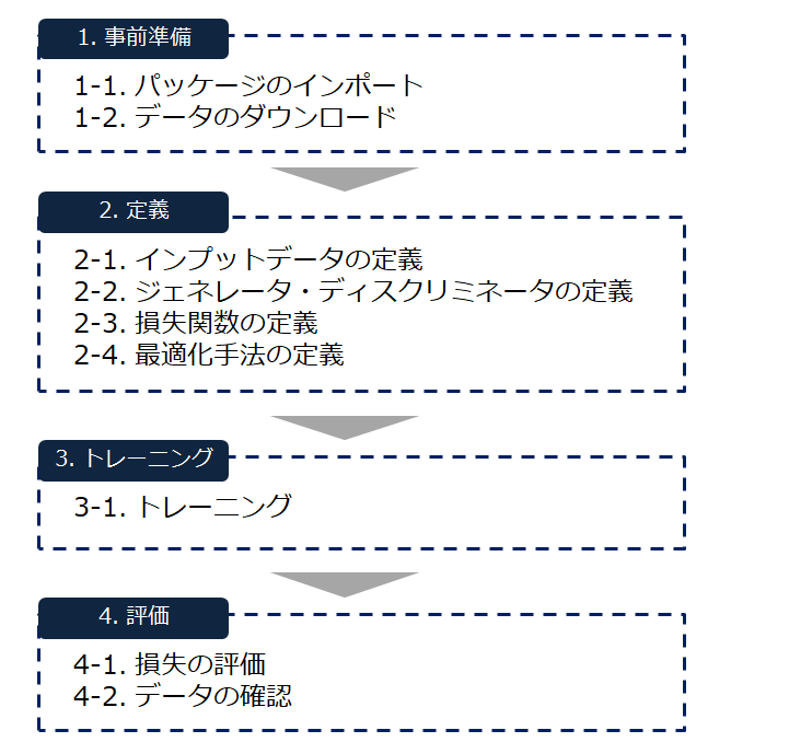
1.事前準備

1-1. パッケージのインポート

%matplotlib inline

import pickle as pkl
import numpy as np
import tensorflow as tf
import matplotlib.pyplot as plt

1-2. データのダウンロード

今回はMNIST(手書き文字)のデータを使用します。

from tensorflow.examples.tutorials.mnist import input_data
mnist = input_data.read_data_sets('MNIST_data')

2.定義

2-1. インプットデータの定義

プレースホルダーを作成する関数を定義します。

def model_inputs(real_dim, z_dim):
    inputs_real = tf.placeholder(tf.float32, (None, real_dim), name='input_real')
    inputs_z = tf.placeholder(tf.float32, (None, z_dim), name='input_z')

    return inputs_real, inputs_z

2-2. ジェネレータ・ディスクリミネータの定義

ジェネレータの定義
Leaky RELUをmax関数で表現しています。

def generator(z,out_dim,n_units=128,reuse=False,alpha=0.01):
    with tf.variable_scope('generator',reuse=reuse):
        h1 = tf.layers.dense(z, n_units, activation=None)#全結合層
        h1 = tf.maximum(alpha * h1, h1) #Leaky RERU

        logits = tf.layers.dense(h1,out_dim,activation=None)#全結合層
        out = tf.tanh(logits)#画像なので-1～1の数字

        return out

ディスクリミネータの定義

def discriminator(x, n_units=128,reuse=False,alpha=0.01):
    with tf.variable_scope('discriminator',reuse=reuse):
        h1 = tf.layers.dense(x, n_units, activation=None)#全結合層
        h1 = tf.maximum(alpha * h1, h1) #Leaky RERU

        logits = tf.layers.dense(h1,1,activation=None)#全結合層
        out = tf.sigmoid(logits)#確率なので0～1の数字

        return out,logits

ハイパパラメータの定義

input_size = 784 #28*28
z_size = 100 #Generatorに与えるランダムベクトルサイズ
g_hidden_size = 128#Generatorの隠れ層のノード数
d_hidden_size = 128#Discriminatorの隠れ層のノード数
alpha = 0.01 #Leaky RELUの傾き
smooth = 0.1 #Discriminatorの学習を円滑にする調整(確率が1に近づきすぎると学習が進まなくなることがあるため、0.9程度に抑えるための変数)

モデルの定義

tf.reset_default_graph()
input_real, input_z = model_inputs(input_size, z_size)

g_model = generator(input_z, input_size, n_units=g_hidden_size, alpha=alpha)

d_model_real, d_logits_real = discriminator(input_real, n_units=d_hidden_size, alpha=alpha)
d_model_fake, d_logits_fake = discriminator(g_model, reuse=True, n_units=d_hidden_size, alpha=alpha)

2-3. 損失関数の定義

d_loss_real = tf.reduce_mean(tf.nn.sigmoid_cross_entropy_with_logits(logits=d_logits_real,
                                            labels=tf.ones_like(d_logits_real)*(1 - smooth)))
d_loss_fake = tf.reduce_mean(tf.nn.sigmoid_cross_entropy_with_logits(logits=d_logits_fake,
                                            labels = tf.zeros_like(d_logits_real)))
d_loss = d_loss_real + d_loss_fake#本物をTrue, 偽物をFalseと判定する精度

#Generator　#偽データが本物として分類されると成功
g_loss = tf.reduce_mean(tf.nn.sigmoid_cross_entropy_with_logits(logits=d_logits_fake,
                                                               labels=tf.ones_like(d_logits_fake)))

2-4. 最適化手法の定義

learning_rate = 0.002

t_vars = tf.trainable_variables()
g_vars = [var for var in t_vars if var.name.startswith('generator')]
d_vars = [var for var in t_vars if var.name.startswith('discriminator')]

d_train_optimize = tf.train.AdamOptimizer(learning_rate).minimize(d_loss, var_list=d_vars)
g_train_optimize = tf.train.AdamOptimizer(learning_rate).minimize(g_loss, var_list=g_vars)

3.トレーニング

3-1. トレーニング

epochs = 100
samples = []
losses = []
saver = tf.train.Saver(var_list=g_vars)#tensorflowの途中経過をファイルに保存する関数。generatorのパラメータ群を保存している。generatorのモデルで画像を生成することが可能になる。
with tf.Session() as sess:
    sess.run(tf.global_variables_initializer())#reset
    for e in range(epochs):
        for i in range(mnist.train.num_examples//batch_size):#各エポックのループ内でミニバッチ学習を行う回数 = サンプル総数/バッチサイズ
            batch = mnist.train.next_batch(batch_size)#ミニバッチ

            batch_images =  batch[0].reshape((batch_size, 784))  #batch_size(100行)*(784列)のデータセット
            batch_images = batch_images * 2 -1 #0~1の濃淡データを-1~1の値に変換。generatorから来るデータとrangeを揃える

            #Generator
            batch_z = np.random.uniform(-1,1,size=(batch_size, z_size))#一様分布

            #トレーニングを実行
            _ = sess.run(d_train_optimize, feed_dict={input_real:batch_images,input_z:batch_z})#最適化計算・パラメータ更新を行う
            _ = sess.run(g_train_optimize, feed_dict={input_z:batch_z})#最適化計算・パラメータ更新を行う
            # _=は、実行はするけど、値を保持しないときに使う

        train_loss_d = sess.run(d_loss,{input_z:batch_z, input_real:batch_images})#トレーニングのロスを計算
        train_loss_g = g_loss.eval({input_z: batch_z})

        print("エポック {}/{} ".format(e+1,epochs),
            "D ロス: {:.4f}".format(train_loss_d),
            "G ロス: {:.4f}".format(train_loss_g))

        losses.append((train_loss_d,train_loss_g))

        sample_z = np.random.uniform(-1,1,size=(16,z_size))
        gen_samples = sess.run(generator(input_z, input_size, n_units=g_hidden_size, reuse=True, alpha=alpha)
                              ,feed_dict={input_z:sample_z})#画像ファイルの生成
        samples.append(gen_samples)
        saver.save(sess,'./checkpoints/generator,ckpt')#途中経過を保存

with open('training_samples.pkl','wb') as f:
    pkl.dump(samples,f)

4.評価

4-1. 損失の評価

収集プロセスを可視化します。

fig, ax = plt.subplots()
losses = np.array(losses)
plt.plot(losses.T[0], label='D')#Dロスのみを取得
plt.plot(losses.T[1], label='G')#Gロスのみを取得
plt.title('Train Loss')
plt.legend()

↓こんな感じで損失関数の推移を可視化できます。

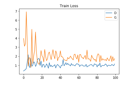
※上記グラフについて
Gはロスが下がっていき、精度が改善されていっている
Dは偽物を偽物としてみる精度があがっているため、なかなか改善されない

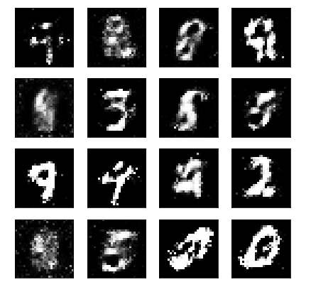
4-2. データの確認

ジェネレータの生成した画像を可視化できます。

#イメージに変換して表示
def view_samples(epoch, samples):
    fig, axes = plt.subplots(figsize=(7,7),nrows=4, ncols=4, sharey=True, sharex=True)
    for ax,img in zip(axes.flatten(),samples[epoch]):
        ax.xaxis.set_visible(False)
        ax.yaxis.set_visible(False)
        im = ax.imshow(img.reshape((28,28)),cmap='Greys_r')
    return fig, axes

with open('training_samples.pkl','rb')as f:
    samples = pkl.load(f)

_ = view_samples(-1, samples)
#samples[-1]なので、最終エポックのデータ

↓こんな感じです。

また、最終エポックだけでなく、学習中の画像データの推移を可視化します。

#10エポックおきに、6個のデータを表示させる
rows,cols = 10, 6
#fig:グラフ全体、axes:個別指定表示要素
fig, axes = plt.subplots(figsize=(7,12), nrows=rows, ncols=cols,sharex=True, sharey=True)

for sample, ax_row in zip(samples[::int(len(samples)/rows)], axes): #サンプル数/10おき
    #100/6 = 15こおきに取り出す
    for img, ax in zip(sample[::int(len(samples)/cols)],ax_row):#::x x分だけインクリメント 指定幅でデータをsamplesから取り出す
        #数字の列を濃淡差として扱い、画像として表示する
        #784個の1次元ベクトルを28*28の2次元行列に変換
        ax.imshow(img.reshape((28,28)),cmap='Greys_r')
        ax.xaxis.set_visible(False)
        ax.yaxis.set_visible(False)

10エポックごとに画像を可視化させています。

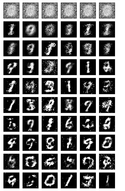
最初はほぼランダムノイズですが、学習していくことで、だんだん人間が判別できる画像になっています。