はじめに
(引き続き初心者向けになります。)
前回は、バーチャルの3D空間と生物学的な観点とのイメージ摺合せやコンピュータ上での3D表現するための3つの座標系について説明しました。
また、そのうちのひとつであるWorld座標系を決定するために、いくつかの行列演算がありそのうちの【回転行列】を説明しました。
今回は、World座標系の平行移動行列と移動行列後に回転行列を掛けるとどうなるのかをイメージ出来ればと思っています。
また、前回の続きとして回転行列を合成した行列の説明から開始して、4次元行列で合わせることですべての行列演算を可能にするところまで説明をします。
4次元の意味は、平行移動の移動量領域です。 (物理空間では時間ですが、3D空間では時間では無いので注意ください。)
では、はじめましょう。
基底ベクトルの変化に伴う各ベクトルの座標や線型写像の行列について
まずは、ここからです。
回転行列により回転すると基底ベクトルが変化します。
よって、基底ベクトルが変化した後の軸を基にした座標を算出する必要があるので、その基礎から入りましょう。
3Dだとイメージしずらいので、2Dで法則を見てみましょう。
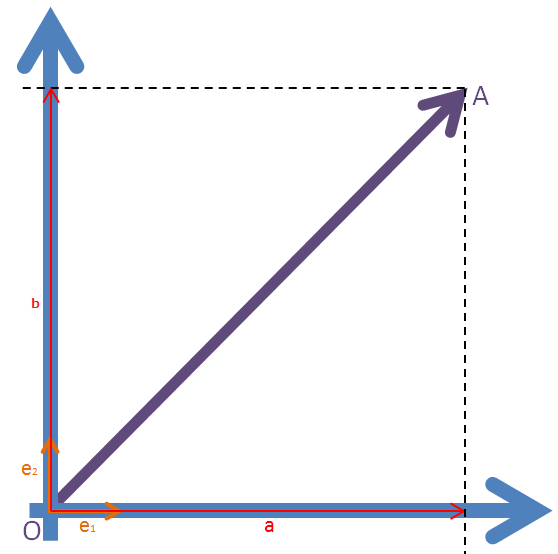
上記の図を数式で表現すると、
\overrightarrow {OA}
=
ae_1 + be_2
 になります。\\
\overrightarrow {OA}上に基底ベクトルを移動した場合の点Aを考えます。\\
基底ベクトルは、(e_1', e_2') = (e_1, e_1 + e_2)に変化したとき\\
e_1 = e_1'\\
e_2 = e_2' - e_1\\
\\
a\overrightarrow {e_1} + b\overrightarrow {e_2} = a\overrightarrow {e_1'} + b(\overrightarrow {e_2'} - \overrightarrow {e_1})\\
= a\overrightarrow {e_1'} + b(\overrightarrow {e_2'} - \overrightarrow {e_1'})\\
= (a - b)\overrightarrow {e_1'} + b\overrightarrow {e_2'}\\
それぞれを行列で表現してみます。
ae_1 + be_2 =
\begin{bmatrix}
e_1 & e_2
\end{bmatrix}
\begin{bmatrix}
a\\
b\\
\end{bmatrix}\\

ae_1 + be_2 =
\begin{bmatrix}
e_1' & e_2'
\end{bmatrix}
\begin{bmatrix}
a - b\\
b\\
\end{bmatrix}
また、
e_1' = e_1\\
e_2' = e_1 + e_2 より\\
\begin{bmatrix}
e_1'\\
e_2'
\end{bmatrix}
=
\begin{bmatrix}
e_1 & e_2
\end{bmatrix}
\begin{bmatrix}
1 & 1\\
0 & 1\\
\end{bmatrix} と表現でき、\\
そこで、
\begin{bmatrix}
1 & 1\\
0 & 1\\
\end{bmatrix}
を Tと置いて、
\begin{bmatrix}
e_1'\\
e_2'
\end{bmatrix}
=
\begin{bmatrix}
e_1 & e_2
\end{bmatrix}
Tとします。\\
\begin{bmatrix}
e_1 & e_2
\end{bmatrix}
T
\begin{bmatrix}
a\\
b\\
\end{bmatrix}
=
\begin{bmatrix}
e_1' & e_2'
\end{bmatrix}
\begin{bmatrix}
a\\
b\\
\end{bmatrix}\\
両辺に行列Tの逆行列を掛けると、
\begin{bmatrix}
e_1 & e_2
\end{bmatrix}
TT^{-1}
\begin{bmatrix}
a\\
b\\
\end{bmatrix}
=
\begin{bmatrix}
e_1' & e_2'
\end{bmatrix}
T^{-1}
\begin{bmatrix}
a\\
b\\
\end{bmatrix}\\
TT^{-1} = 1なので、\\
\begin{bmatrix}
e_1 & e_2
\end{bmatrix}
\begin{bmatrix}
a\\
b\\
\end{bmatrix}
=
\begin{bmatrix}
e_1' & e_2'
\end{bmatrix}
T^{-1}
\begin{bmatrix}
a\\
b\\
\end{bmatrix}となる。\\
元の基底ベクトル(e_1 \  e_2)のとき、
\begin{bmatrix}
a\\
b\\
\end{bmatrix}と表されるベクトルは、
変化後の基底ベクトル(e_1' \  e_2')のとき、
T^{-1}
\begin{bmatrix}
a\\
b\\
\end{bmatrix}となる。\\
ここで、元の基底行列における変換行列をAとおき説明する。
元の基底ベクトル(e_1 \  e_2)のとき、
\begin{bmatrix}
e_1 & e_2
\end{bmatrix}A
\begin{bmatrix}
x\\
y
\end{bmatrix}となる。\\
基底ベクトルが(e_1' \ e_2')に変化した時は、
\begin{bmatrix}
e_1 & e_2
\end{bmatrix}A
\begin{bmatrix}
x\\
y
\end{bmatrix}=
\begin{bmatrix}
e_1' & e_2'
\end{bmatrix}T^{-1} A
\begin{bmatrix}
x\\
y
\end{bmatrix}となる。\tag{1} \\
ここで、T^{-1}\begin{bmatrix}
x\\
y
\end{bmatrix}を
\begin{bmatrix}
x'\\
y'
\end{bmatrix}とおく\\
すなわち、
T^{-1}\begin{bmatrix}
x\\
y
\end{bmatrix}=
\begin{bmatrix}
x'\\
y'
\end{bmatrix}とする\\
両辺にTを掛けて \
TT^{-1}\begin{bmatrix}
x\\
y
\end{bmatrix}=
T\begin{bmatrix}
x'\\
y'
\end{bmatrix}\\
TT^{-1}は、1なので\\
\begin{bmatrix}
x\\
y
\end{bmatrix}=
T\begin{bmatrix}
x'\\
y'
\end{bmatrix}となる\\
上記式を(1)式に代入すると、\\
\begin{bmatrix}
e_1 & e_2
\end{bmatrix}A
\begin{bmatrix}
x\\
y
\end{bmatrix}=
\begin{bmatrix}
e_1' & e_2'
\end{bmatrix}T^{-1} A T
\begin{bmatrix}
x'\\
y'
\end{bmatrix}となり、
線形写像を表す行列は、T^{-1} A T \ となることが分かる。
すべての軸回転を考慮した回転行列を算出する
ロール・ピッチ・ヨーの順で回転させる場合の行列の計算順序について、上記の線形写像を表す行列式を基に算出し3軸すべてを統合した回転行列を求める。
まず、ロール・ピッチ・ヨー行列をそれぞれRotationのRとroll, pitch, yawの頭文字を付けて行列として表現します。
VRで一般的なエンジンは、UnityなのでUnityの仕様に合わせるとroll(Y軸), pitch(X軸), yaw(Z軸)となります。
Rotation \ Matrix \ of \ Roll \ Axis: \ R_r\\
Rotation \ Matrix \ of \ Pitch \ Axis: \ R_p\\
Rotation \ Matrix \ of \ Yaw \ Axis: \ R_y
Z軸⇒X軸⇒Y軸の順に回転させるイメージで解説します。
基底ベクトルを(e_1 \ e_2 \ e_3)とする。\\
Z軸に回転する行列は、\\
R =
\begin{bmatrix}
e_1 & e_2 & e_3
\end{bmatrix} R_r\\
Z軸を中心に回転することで基底ベクトルが変化したので、
基底ベクトルを(e_1 \ e_2 \ e_3)R_rとする。\\
線形写像ベクトルは、\\
R_r^{-1} R_p R_r \ となります。\\
R =
\begin{bmatrix}
e_1 & e_2 & e_3
\end{bmatrix} R_r R_r^{-1} R_p R_r \\
R_r R_r^{-1}は、1になるので\\
R =
\begin{bmatrix}
e_1 & e_2 & e_3
\end{bmatrix}R_p R_rとなる
Z軸⇒X軸を中心に回転することで基底ベクトルが変化したので、
基底ベクトルを(e_1 \ e_2 \ e_3)R_p R_rとする。\\
線形写像ベクトルは、\\
(R_p R_r)^{-1} R_y (R_p R_r) \ となり、\\
R =
\begin{bmatrix}
e_1 & e_2 & e_3
\end{bmatrix} (R_p R_r) (R_p R_r)^{-1} R_y (R_p R_r) \\
(R_p R_r) (R_p R_r)^{-1}は、1になるので\\
R =
\begin{bmatrix}
e_1 & e_2 & e_3
\end{bmatrix}R_y R_p R_rとなる
ようするに、回転させたい軸とは逆順に掛ける事で期待する回転行列を得られることを
理解できたと思います。
この結果を基に、ヨー * ピッチ * ロールの順に掛けていくと回転行列が完成します。
行列で展開すると以下の式になります。\\
\begin{bmatrix}
x \\ y \\ z \\ 1 \\
\end{bmatrix} =
\begin{bmatrix}
\cos \theta_y & -\sin \theta_y & 0 & 0 \\
\sin \theta_y & \cos \theta_y & 0 & 0 \\
0 & 0 & 1 & 0 \\
0 & 0 & 0 & 1 \\
\end{bmatrix}
\begin{bmatrix}
1 & 0 & 0 & 0 \\
0 & \cos \theta_p & -\sin \theta_p & 0 \\
0 & \sin \theta_p & \cos \theta_p & 0 \\
0 & 0 & 0 & 1 \\
\end{bmatrix}
\begin{bmatrix}
\cos \theta_r & 0 & \sin \theta_r & 0 \\
0 & 1 & 0 & 0 \\
-\sin \theta_r & 0  & \cos \theta_r & 0 \\
0 & 0 & 0 & 1 \\
\end{bmatrix}\\
順番に解いていきましょう。\\
=
\begin{bmatrix}
\cos \theta_y & -\sin \theta_y \cos \theta_p & \sin \theta_y \sin \theta_p & 0 \\
\sin \theta_y & \cos \theta_y \cos \theta_p & -\cos \theta_y \sin \theta_p  & 0 \\
0 & \sin \theta_p & \cos \theta_p & 0 \\
0 & 0 & 0 & 1 \\
\end{bmatrix}
\begin{bmatrix}
\cos \theta_r & 0 & \sin \theta_r & 0 \\
0 & 1 & 0 & 0 \\
-\sin \theta_r & 0  & \cos \theta_r & 0 \\
0 & 0 & 0 & 1 \\
\end{bmatrix}\\
=
\begin{bmatrix}
\cos \theta_y \cos \theta_r - \sin \theta_y \sin \theta_p \sin \theta_r & -\sin \theta_y \cos \theta_p & \cos \theta_y \sin \theta_r + \sin \theta_y \sin \theta_p \cos \theta_r & 0 \\
\sin \theta_y \cos \theta_r + \cos \theta_y \sin \theta_p \sin \theta_r & \cos \theta_y \cos \theta_p & \sin \theta_y \sin \theta_r -\cos \theta_y \sin \theta_p \cos \theta_r & 0 \\
-\sin \theta_p \sin \theta_r & \sin \theta_p & \cos \theta_p \cos \theta_r & 0 \\
0 & 0 & 0 & 1 \\
\end{bmatrix}\\
となります。
基底行列に上記の行列を掛ける事で、向きを変える事が出来ます。
※画像では、説明しづらい部分ですので数式での説明となります。ご了承ください。
平行移動行列について
3D空間における移動を行列で表現します。
平行移動とは、原点からの相対移動距離になります。
例えば、ax + by + cz = 0 というベクトルがあります。
x, y, z軸方向にそれぞれ、⊿x, ⊿y, ⊿zだけ移動したとする。
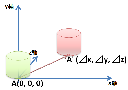
基底行列を(x, y, z)とすると
式は、\\
X' = x * 1 + y * 0 + z * 0 + \Delta x\\
Y' = x * 0 + y * 1 + z * 0 + \Delta y\\
Z' = x * 0 + y * 0 + z * 1 + \Delta z\\
となるので、行列に直すと\\
\begin{bmatrix}
X' \\ Y' \\ Z' \\ 1
\end{bmatrix} =
\begin{bmatrix}
x & y & z & 1
\end{bmatrix}
\begin{bmatrix}
1 & 0 & 0 & \Delta x \\
0 & 1 & 0 & \Delta y \\
0 & 0 & 1 & \Delta z \\
0 & 0 & 1 & 1 \\
\end{bmatrix}
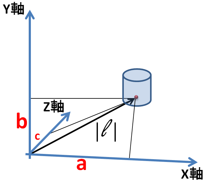
平行移動後の回転について
平行移動後の回転行列は、何を表現するかと言うと基底行列を中心にして平行移動した移動量を半径とすし、
円周上を回転する行列のことです。
イメージを図で表すと、以下の通りとなります。
a, b, cは、それぞれX軸、Y軸、Z軸方向の長さになります。
|l| = a + b + c
まず、移動した後の基底ベクトルと座標があり、
これに回転行列を掛けるということは、各軸の原点を中心に半径|l|の球面上に沿って円錐を動かす
イメージになります。
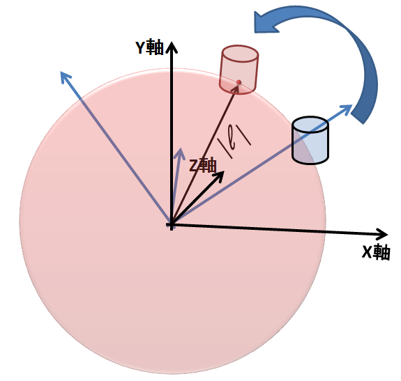
回転行列には、変化は無いです。
一応、書いておきます。
R_yR_pR_y =
\begin{bmatrix}
x \\ y \\ z \\ 1 \\
\end{bmatrix}
=
\begin{bmatrix}
\cos \theta_y \cos \theta_r - \sin \theta_y \sin \theta_p \sin \theta_r & -\sin \theta_y \cos \theta_p & \cos \theta_y \sin \theta_r + \sin \theta_y \sin \theta_p \cos \theta_r & 0 \\
\sin \theta_y \cos \theta_r + \cos \theta_y \sin \theta_p \sin \theta_r & \cos \theta_y \cos \theta_p & \sin \theta_y \sin \theta_r -\cos \theta_y \sin \theta_p \cos \theta_r & 0 \\
-\sin \theta_p \sin \theta_r & \sin \theta_p & \cos \theta_p \cos \theta_r & 0 \\
0 & 0 & 0 & 1 \\
\end{bmatrix}\\
回転行列をそれぞれ、R_r, R_p, R_yとする。\\
また、平行移動行列をTとする。\\
基底行列(e_1 \ e_2 \ e_3)から回転 * 移動したときの基底行列は、\\
(e_1 \ e_2 \ e_3)(TR_{y1}R_{p1}R_{y1})^{-1}(TR_{y1}R_{p1}R_{y1})(R_{y2}R_{p2}R_{y2})(TR_{y1}R_{p1}R_{y1}) \ となる\\
(TR_{y1}R_{p1}R_{y1})^{-1}(R_{y1}R_{p1}R_{y1})は、1になるので\\
(e_1 \ e_2 \ e_3)R_{y2}R_{p2}R_{y2}TR_{y1}R_{p1}R_{y1}
言葉で表現すると、
(移動後の回転行列) (平行移動行列) (回転行列)
という順番で掛け算をすることになる。
まとめ
3D上での位置決めは、基底行列も変化するので前の位置と連動する場合は
前のオブジェクトの位置行列を基底行列としてオブジェクトの位置決定を行えば良い。
※この部分だけで関節の連結方法については理解できると思います。
次回は、クォータニオン補間を使った回転などを説明します。(寄り道です)
関節の連結を考えたクラス設計なども説明していきます。 (読者が最終的に求めているのはここでしょうから・・・)
間違いや疑問点ありましたら、遠慮なくどうぞ。
ちょっと、今回は難しいかもしれません。