本スライドは、重力プログラミング入門「第2回:重力波を解析する」の登壇向けスライドです
![]()
![]() 続編(?)、重力プログラミング入門「第3回:太陽フレアをディープラーニングで予測する」も公開
続編(?)、重力プログラミング入門「第3回:太陽フレアをディープラーニングで予測する」も公開
はじめに
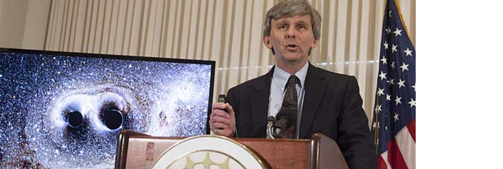
100年間、その存在を確認できなかったのに、2015年9月以降、立て続けに5回も観測された
「重力波」をプログラムで解析してみたいと思います ![]()
タイトルが「第2回」となっているのは、2017/9の福岡数学イベントで登壇した、
重力プログラミング入門「第1回:地球の重力下で人工衛星を公転軌道に乗せる」の続編(?)のためです ![]()
なお、Twitterでは、ハッシュタグ#QuaUnivFukuoka にて、重力や宇宙、数学・物理学関連のネタをつぶやいてますので、フォローいただけたら幸いです ![]()
重力波とは?
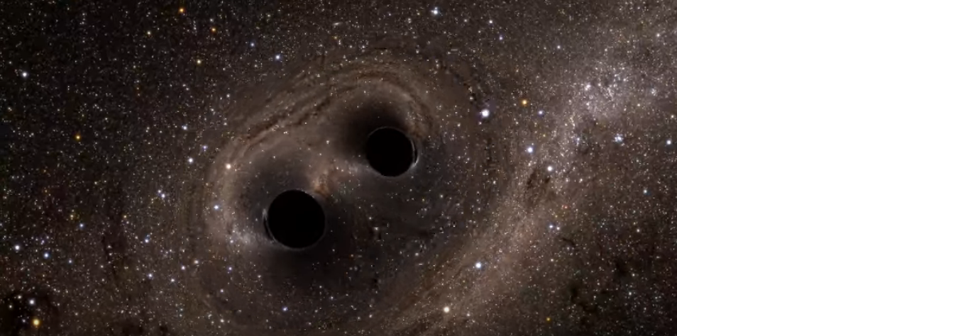
重力波は、巨大質量の天体(ブラックホール、中性子星など)が運動することで、天体の「時空の歪み」が波として伝わる現象を指します
天体の運動?、と言われてもピンと来ない方も多いと思うので、以下の動画で、2つのブラックホールが合体する様をご覧いただき、イメージを掴んでください ![]()
https://www.youtube.com/watch?v=I_88S8DWbcU
重力の理論である「一般相対性理論」を提唱したアインシュタインが、1916年に重力波の存在を予言していたものの、つい最近まで、実際に観測されることはありませんでした
そして、予言からちょうど100年後の「2015/09/14 09:50:45」、初めて重力波が観測されました ![]()
「重力」=メカニズム不明の「万有引力」だった頃
重力波の元である「重力」は、紀元前350年頃の古代ギリシャ初期から議論されており、天動説から地動説への変遷と共に、様々なパラダイムが移り変わっていきました
その中でも最もメジャーなのが、ニュートンが1687年にまとめた「万有引力の法則」と、ホイヘンスが発見した「遠心力の公式」で導出される「自転の遠心力」を引いた合力を「重力」とする考え方です
なお天文学や宇宙開発では、「重力」≒「万有引力」として扱っており、自転による遠心力は省略されるようです
「万有引力」の数式は、以下の通りです ※Qiita数式機能、SymPyより書きやすい ![]()
F=G\frac{Mm}{r^2}
(この数式の内容は、第1回 重力プログラミング入門 のP26で解説しています)
高校の頃に習いますが覚えてますか?
私は重力に携わるまでの十数年前まで、スッカリ忘れていました… ![]()
「万有引力の法則」は、発見から300年以上、支持されましたが、実はそのメカニズムは証明されないままでした
「重力」=「時空の歪み」であると分かった頃
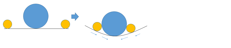
1916年、アインシュタインにより「一般相対性理論」が発表され、「万有引力」のメカニズムも、ある物体が質量により時空(≒3次元空間に時間を加えた概念)を歪めたことで、もう一方の物体が、歪んだ方向に転がっていく現象であると分かりました
これを数式で表したのが、「重力場の方程式」、別名「アインシュタイン方程式」と呼ばれるものです
G_{μν}=\frac{8πG}{c^4}T_{μν}
数式の各項は以下の通りです
- Gμν:「アインシュタイン・テンソル」と呼ばれる、時空の曲がり具合
- G:「重力定数」と呼ばれる、重力の大きさを表すもの ※万有引力の法則のGと同じ
- c:光の速度
- Tμν:「エネルギー・運動量テンソル」と呼ばれる、質量・エネルギーの密度と流れを表すもの
この数式から、「時空の歪み」が「エネルギー場」と釣り合うことが分かります
重力波の正体
重力波とは、重力場の方程式で出てきた、「時空の歪み」が、波として伝わっていく現象であり、イメージにすると、以下のような感じになります
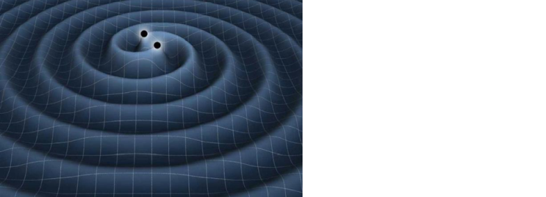
この波の規模は、「10のマイナス21乗」とかなり小さく、これは「地球から太陽の距離で、水素原子1つ分が歪む」程度の微小な変化でしかありません
100年間、重力波を観測できなかったのは、このような微小な変化を捉えるための技術が無かったことが、主な要因だと考えられています ![]()
重力波を観測するための技術
この100年でコンピュータは飛躍的に進歩し、科学技術もその恩恵で発展し、精密な装置開発が可能となりました
その結果、「地球から太陽の距離で、水素原子1つ分が歪む」程度の微小な変化も検出できるようになりましたが、具体的にどんな技術が使われているのでしょう? ![]()
レーザー干渉計
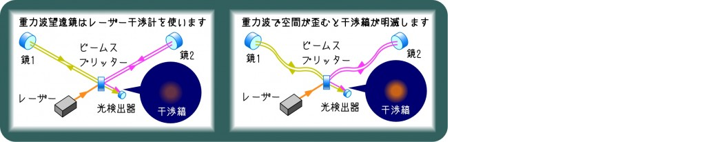
2本のL字パイプの先端の鏡にレーザーを当て、跳ね返りを検出器で拾うと、通常は、レーザーが同じタイミングで戻りますが、重力波で空間が歪むと、光が曲がるため、僅かに到達がズレるので、これで重力波を検出します ![]()
LIGOレーザー干渉計重力波天文台
重力波による歪みは、前述の通り、とても小さいため、非常に大きなレーザー干渉計装置が必要となります
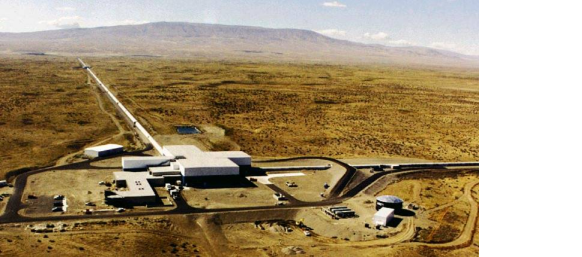
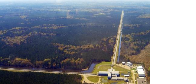
今回、初めて重力波を検出したのは、LIGO(Laser Interferometer Gravitational-Wave Observatory:レーザー干渉計重力波観測所)と呼ばれる、ワシントン州ハンフォード(アメリカ東海岸側)と、ルイジアナ州リビングストン(アメリカ西海岸側)の2ヵ所にある施設です
パイプ1本の長さが4Kmもある、巨大な観測施設によって、初めて観測可能となった訳です ![]()
ワシントン州ハンフォード観測所
ルイジアナ州リビングストン観測所
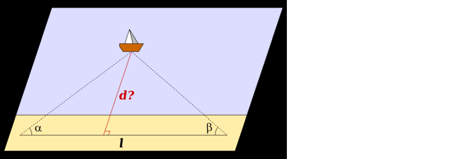
また各施設間は、3,002km離れている(≒光速にすると約10ミリ秒の距離がある)ため、2つの施設への重力波到達の僅かな時間のズレから、三角測量を応用して重力波の発生源を位置特定することが可能です
重力波から分かったこと
LIGOの2つの観測所で、重力波はほぼ同時に観測され、振幅の大きさや波形が、同じような形をしていたことから、ノイズでは無く、重力波の影響であることが特定できました
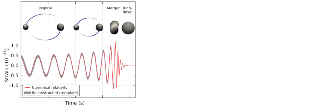
キャッチした波形は、研究チームが予測した、2つのブラックホールが徐々に近づき、近づくにつれて重力波の周期も狭まり、合体する際には大きな振幅と周期の短縮が起こり、合体後は運動が無くなることで振幅も無くなる、という予測通りの観測結果でした(太陽の35倍と29倍の質量を持つブラックホールが合体した、まで分かっています)
重力波解析のための開発環境準備
それでは実際に、LIGO観測所で計測されたデータを手元で解析するために開発環境を揃えます ![]()
事前準備①:Python 3.xのインストール
Anacondaを使うと、Pythonおよび関連ライブラリのインストールが簡単になります
Anacondaのインストール方法は、AI入門「第3回:数学が苦手でも作って使えるKerasディープラーニング」という別シリーズでも扱っており、こちらのP13~P16をご参考ください

事前準備②:必要ライブラリのインストール
スライドP16の手順で起動したターミナル上で、以下コマンドを入力していきます
pip install numpy
pip install scipy
pip install matplotlib
pip install h5py
各ライブラリは、Pythonで科学計算をする際に、比較的メジャーなライブラリなので、ググれば何者かは調べられます ![]()
事前準備③:Jupyter Notebookの起動
「Jupyter Notebook」と呼ぶ、ブラウザ上での開発環境をターミナルから起動できます
mkdir -p 【任意の場所で、任意のフォルダ名】
cd 【上記の場所・フォルダ名】
jupyter notebook
ここでは、「/piacere/code/ligo」というフォルダ名を使います
mkdir -p /piacere/code/ligo
cd /piacere/code/ligo
jupyter notebook
重力波を解析してみる
2ヵ所のLIGO観測所が計測したデータを使い、重力波が予測通りだったのかを、セットアップしたJupyter Notebookにて解析していきます
今回、解析対象とするのは、LIGOでオープンになっているデータのうち、最も最新の2017年1月に観測されたデータ「GW170104」という、地球から最も離れた場所で発生した、3例目の重力波です(ブラックホールの規模は、太陽の31倍と19倍の質量)
LIGOから観測データと解析プログラムを入手する
LIGOが公開しているデータは、解析過程を全て記述したJupyter Notebookおよび解析プログラムのPythonコードがセットになって配布されているため、これを入手します
以下URLを別タブでクリックし、「Download the data on a computer with a python installation」というセクションにあるリンク「LOSC_Event_tutorial.zip」をクリックして、手元にダウンロードしてください
これを、先ほど作成したフォルダ内に展開します(展開後のJupyter Notebookは以下のようになります)
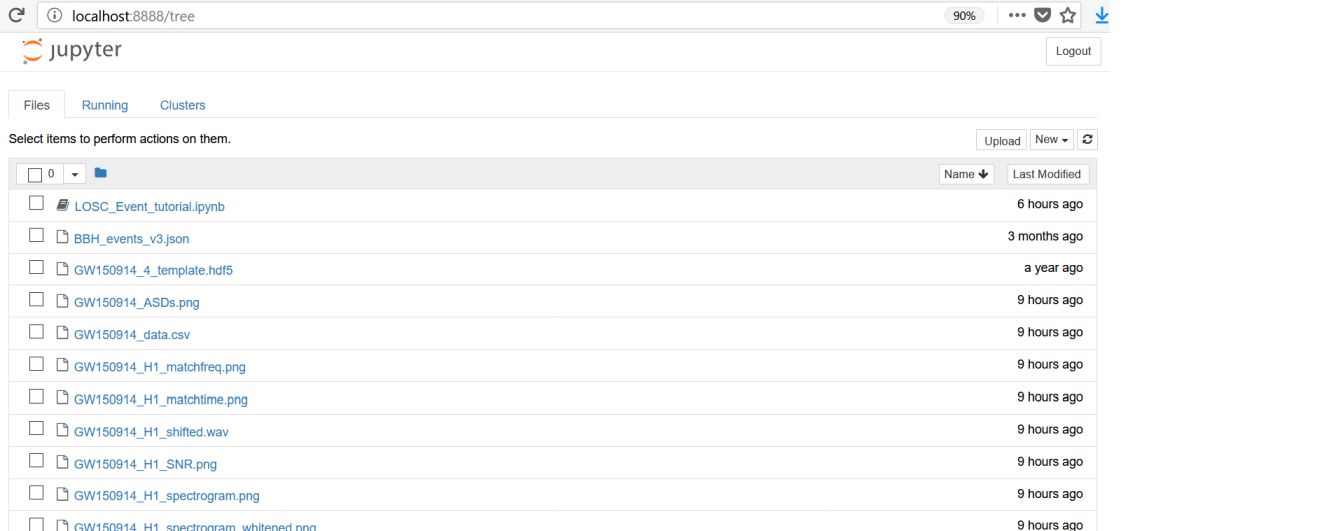
なお、展開した中身のファイルを作成フォルダ直下に置いていない場合、この後Jupyter Notebookで実行する際に、以下のエラーが出ますので、エラーが出た際は、作成フォルダ直下にファイルを展開するようにしてください
AttributeError: module 'readligo' has no attribute 'loaddata'
Jupyter Notebookの起動が、作成フォルダ直下で無い場合も、同じエラーが出るので、その際は、作成フォルダに移動し直して、Jupyter Notebookを起動してください
ちなみに、このエラーの原因は、import時にreadligo.pyが見つからないことが原因で、ターミナルでは以下エラーで判別できるものの、Jupyter Notebookでは、いずれのケースでもimport時では無く、利用時に上記エラーでしか表示されないため、パッと見ではエラー判別できません
import readligo as rl
Traceback (most recent call last):
  File "<stdin>", line 1, in <module>
ModuleNotFoundError: No module named 'readligo'
Python 3.xで動かない箇所の修正
展開した解析プログラムは、Python 2.xでの動作を想定したプログラムのため、一部、Python 3.xで以下エラーが発生し、動かないため、修正が必要です
TabError: inconsistent use of tabs and spaces in indentation
「readligo.py」というファイルを開き、412行目に行くと、タブ文字が混入しており、Python 2.xでは無視される一方、Python 3.xではエラーとなるため、半角スペースに書き換えます
測定データの読み込み
「LOSC_Event_tutorial.ipynb」をクリックし、下の方にスクロールしていくと、データ入力が可能な、灰色背景のブロックが出てきますが、こちらが解析プログラムです ![]()
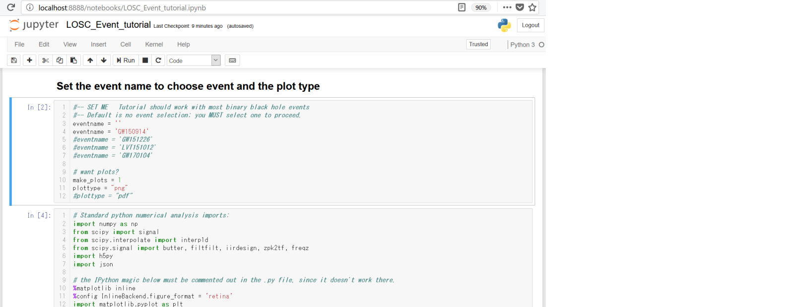
今回、「観測した重力波が予測通りか?」のみ確認するため、そこに該当しない解析は省略しますが、早速、変数定義とimportの2ブロックは省略し、その後の観測データ設定読込から解説します
# Read the event properties from a local json file
fnjson = "BBH_events_v3.json"
try:
    events = json.load(open(fnjson,"r"))
except IOError:
    print("Cannot find resource file "+fnjson)
    print("You can download it from https://losc.ligo.org/s/events/"+fnjson)
    print("Quitting.")
    quit()

# did the user select the eventname ?
try:
    events[eventname]
except:
    print('You must select an eventname that is in '+fnjson+'! Quitting.')
    quit()
「BBH_events_v3.json」には、過去4回分の観測データ設定が入っており、今回の「GW170104」は、以下の通りです
{
  "GW170104":{
      "name":"GW170104",
      "fn_H1"       : "H-H1_LOSC_4_V1-1167559920-32.hdf5",
      "fn_L1"       : "L-L1_LOSC_4_V1-1167559920-32.hdf5",
      "fn_template" : "GW170104_4_template.hdf5",
      "fs"          : 4096,
      "tevent"      : 1167559936.6,
      "utcevent"    : "2017-01-04T10:11:58.60",
      "m1"          : 33.64,
      "m2"          : 24.82,
      "a1"          : -0.236,
      "a2"          : 0.024,
      "approx"      : "lalsim.SEOBNRv2",
      "fband"       : [43.0,800.0],
      "f_min"       : 10.0
  }
}
「GW170104_4_template.hdf5」は、予測波形データが、HDF5フォーマットで格納されており、「H-H1_LOSC_4_V1-1167559920-32.hdf5」「L-L1_LOSC_4_V1-1167559920-32.hdf5」には、それぞれはハンフォード観測所分、リビングストン観測所分のデータが入っています
「fs」はサンプリングレート、「tevent」は発生日時、「fband」はバンドパス周波数帯です
# Extract the parameters for the desired event:
event = events[eventname]
fn_H1 = event['fn_H1']              # File name for H1 data
fn_L1 = event['fn_L1']              # File name for L1 data
fn_template = event['fn_template']  # File name for template waveform
fs = event['fs']                    # Set sampling rate
tevent = event['tevent']            # Set approximate event GPS time
fband = event['fband']              # frequency band for bandpassing signal
print("Reading in parameters for event " + event["name"])
print(event)
ハンフォード観測所のデータと、リビングストン観測所のデータを読み込みます
#----------------------------------------------------------------
# Load LIGO data from a single file.
# FIRST, define the filenames fn_H1 and fn_L1, above.
#----------------------------------------------------------------
try:
    # read in data from H1 and L1, if available:
    strain_H1, time_H1, chan_dict_H1 = rl.loaddata(fn_H1, 'H1')
    strain_L1, time_L1, chan_dict_L1 = rl.loaddata(fn_L1, 'L1')
except:
    print("Cannot find data files!")
    print("You can download them from https://losc.ligo.org/s/events/"+eventname)
    print("Quitting.")
    quit()
各データの件数、最小、平均、最大を表示します
# both H1 and L1 will have the same time vector, so:
time = time_H1
# the time sample interval (uniformly sampled!)
dt = time[1] - time[0]

# Let's look at the data and print out some stuff:

print('time_H1: len, min, mean, max = ', \
    len(time_H1), time_H1.min(), time_H1.mean(), time_H1.max() )
print('strain_H1: len, min, mean, max = ', \
    len(strain_H1), strain_H1.min(),strain_H1.mean(),strain_H1.max())
print( 'strain_L1: len, min, mean, max = ', \
    len(strain_L1), strain_L1.min(),strain_L1.mean(),strain_L1.max())

#What's in chan_dict?  (See also https://losc.ligo.org/tutorials/)
bits = chan_dict_H1['DATA']
print("For H1, {0} out of {1} seconds contain usable DATA".format(bits.sum(), len(bits)))
bits = chan_dict_L1['DATA']
print("For L1, {0} out of {1} seconds contain usable DATA".format(bits.sum(), len(bits)))
測定データ(ノイズ入り)のプロット
各データをグラフ表示します
# plot +- deltat seconds around the event:
# index into the strain time series for this time interval:
deltat = 5
indxt = np.where((time >= tevent-deltat) & (time < tevent+deltat))
print(tevent)

if make_plots:
    plt.figure()
    plt.plot(time[indxt]-tevent,strain_H1[indxt],'r',label='H1 strain')
    plt.plot(time[indxt]-tevent,strain_L1[indxt],'g',label='L1 strain')
    plt.xlabel('time (s) since '+str(tevent))
    plt.ylabel('strain')
    plt.legend(loc='lower right')
    plt.title('Advanced LIGO strain data near '+eventname)
    plt.savefig(eventname+'_strain.'+plottype)
赤線がハンフォード観測所、緑線がリビングストン観測所のデータを表します
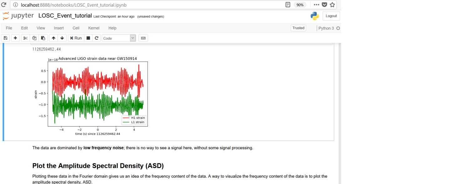
この波形は、予測波形と似ても似つかないのですが、これは多くのノイズを含んでいるためです ![]()
測定データから重力波のみを取り出す
重力波のデータから読み取るべきことは、「一瞬の変化」であるため、データ全体にまんべんなく入っているようなノイズを除外する必要があります
そのために、「白色化」という、各周波数成分への分解と正規化によるノイズ除去手法を用います
また、そもそもノイズと見なせる特定周波数帯も除外します
データを各周波数成分に分解する
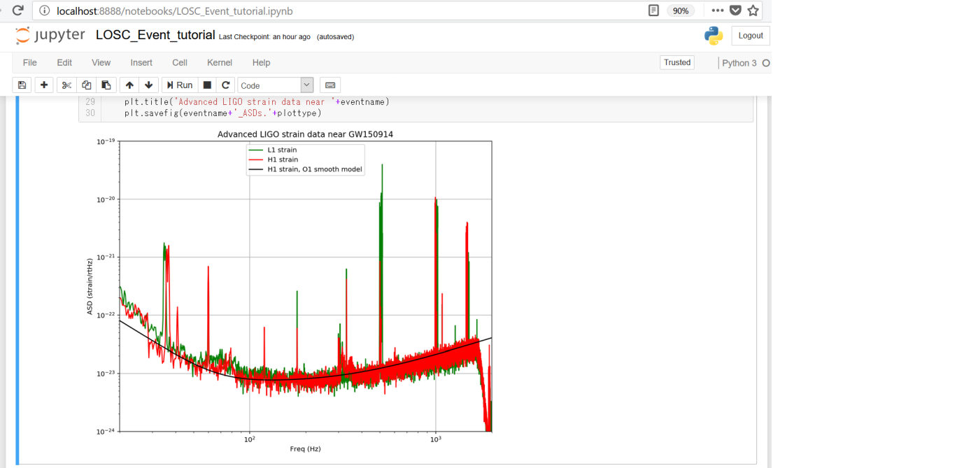
まず、各周波数成分の分布をビジュアル化してみますが、これには、振幅スペクトル密度(ASD:Amplitude Spectral Density)をプロットしてみます
振幅スペクトル密度は、パワースペクトル密度(mlab.psd())のルートで計算できます
またプロットの際、下限周波数を20Hz、上限周波数を2,000Hzとします
20Hzの方は、LIGOが、20Hz未満の検出にてノイズが非常に高いためです
2,000Hzの方については、「ナイキスト周波数」と呼ばれる、サンプリングレートの半分を超える周波数成分が折り返す現象により、元の信号として再現されないため、fs=4,096Hzの半分である2,048Hzより少し下でカットします
make_psds = 1
if make_psds:
    # number of sample for the fast fourier transform:
    NFFT = 4*fs
    Pxx_H1, freqs = mlab.psd(strain_H1, Fs = fs, NFFT = NFFT)
    Pxx_L1, freqs = mlab.psd(strain_L1, Fs = fs, NFFT = NFFT)

    # We will use interpolations of the ASDs computed above for whitening:
    psd_H1 = interp1d(freqs, Pxx_H1)
    psd_L1 = interp1d(freqs, Pxx_L1)

    # Here is an approximate, smoothed PSD for H1 during O1, with no lines. We'll use it later.
    Pxx = (1.e-22*(18./(0.1+freqs))**2)**2+0.7e-23**2+((freqs/2000.)*4.e-23)**2
    psd_smooth = interp1d(freqs, Pxx)
if make_plots:
    # plot the ASDs, with the template overlaid:
    f_min = 20.
    f_max = 2000.
    plt.figure(figsize=(10,8))
    plt.loglog(freqs, np.sqrt(Pxx_L1),'g',label='L1 strain')
    plt.loglog(freqs, np.sqrt(Pxx_H1),'r',label='H1 strain')
    plt.loglog(freqs, np.sqrt(Pxx),'k',label='H1 strain, O1 smooth model')
    plt.axis([f_min, f_max, 1e-24, 1e-19])
    plt.grid('on')
    plt.ylabel('ASD (strain/rtHz)')
    plt.xlabel('Freq (Hz)')
    plt.legend(loc='upper center')
    plt.title('Advanced LIGO strain data near '+eventname)
    plt.savefig(eventname+'_ASDs.'+plottype)
赤線がハンフォード観測所分、緑線がリビングストン観測所分、黒線がハンフォード観測所分を平滑化したものとなります
白色化とバンドパスフィルタ
「Binary Neutron Star (BNS) detection range」のブロックを読み飛ばし(中性子星とか面白そうではありますが…)、「Whitening」というタイトルの、データを白色化するコードに進みます
白色化の処理としては、フーリエ変換(np.fft.rfft())で元データを各周波数成分に分解し、振幅スペクトル密度で除算することで正規化し、その後、逆フーリエ変換(np.fft.irfft())で元に戻すことで、データ全体にまんべんなく入っている波ほど目立たなくなり、「一瞬の変化」の波が強調されるようになります
白色化の後、高周波ノイズが残っているので、バンドパスフィルタで除去します
def whiten(strain, interp_psd, dt):
    Nt = len(strain)
    freqs = np.fft.rfftfreq(Nt, dt)
    freqs1 = np.linspace(0,2048.,Nt/2+1)

    # whitening: transform to freq domain, divide by asd, then transform back,
    # taking care to get normalization right.
    hf = np.fft.rfft(strain)
    norm = 1./np.sqrt(1./(dt*2))
    white_hf = hf / np.sqrt(interp_psd(freqs)) * norm
    white_ht = np.fft.irfft(white_hf, n=Nt)
    return white_ht

whiten_data = 1
if whiten_data:
    # now whiten the data from H1 and L1, and the template (use H1 PSD):
    strain_H1_whiten = whiten(strain_H1,psd_H1,dt)
    strain_L1_whiten = whiten(strain_L1,psd_L1,dt)

    # We need to suppress the high frequency noise (no signal!) with some bandpassing:
    bb, ab = butter(4, [fband[0]*2./fs, fband[1]*2./fs], btype='band')
    normalization = np.sqrt((fband[1]-fband[0])/(fs/2))
    strain_H1_whitenbp = filtfilt(bb, ab, strain_H1_whiten) / normalization
    strain_L1_whitenbp = filtfilt(bb, ab, strain_L1_whiten) / normalization
観測データと予測波形のプロット
「Spectrograms」の2ブロックは飛ばして、「Waveform Template」というタイトルが付いた、予測波形(コード中はtemplateというキーワードを使用)の読み込みを行います
# read in the template (plus and cross) and parameters for the theoretical waveform
try:
    f_template = h5py.File(fn_template, "r")
except:
    print("Cannot find template file!")
    print("You can download it from https://losc.ligo.org/s/events/"+eventname+'/'+fn_template)
    print("Quitting.")
    quit()
その次のブロックの「extract metadata from the template file」で始まるコードは、ほぼ実行不要なので、以下のみ手入力して実行します
# extract metadata from the template file:
template_p, template_c = f_template["template"][...]

# the template extends to roughly 16s, zero-padded to the 32s data length. The merger will be roughly 16s in.
template_offset = 16.
タイトルが「Matched filtering to find the signal」のブロックで、観測された重力波と予測波形をプロットしていますが、その2つ以外のプロットが多くあるので、こちらも以下のみ手入力して実行します
ちなみに、予測波形には、各観測波形に合わせるためのシフトを行い、白色化とバンドパスフィルタによる高周波ノイズ除去を行っています
# -- To calculate the PSD of the data, choose an overlap and a window (common to all detectors)
#   that minimizes "spectral leakage" https://en.wikipedia.org/wiki/Spectral_leakage
NFFT = 4*fs
psd_window = np.blackman(NFFT)
NOVL = NFFT/2    # and a 50% overlap:
# define the complex template, common to both detectors:
template = (template_p + template_c*1.j)
# We will record the time where the data match the END of the template.
etime = time+template_offset
# the length and sampling rate of the template MUST match that of the data.
datafreq = np.fft.fftfreq(template.size)*fs
df = np.abs(datafreq[1] - datafreq[0])

# to remove effects at the beginning and end of the data stretch, window the data
# https://en.wikipedia.org/wiki/Window_function#Tukey_window
try:   dwindow = signal.tukey(template.size, alpha=1./8)  # Tukey window preferred, but requires recent scipy version
except: dwindow = signal.blackman(template.size)          # Blackman window OK if Tukey is not available

# prepare the template fft.
template_fft = np.fft.fft(template*dwindow) / fs
# loop over the detectors
dets = ['H1', 'L1']
for det in dets:

    if det is 'L1': data = strain_L1.copy()
    else:           data = strain_H1.copy()

    # -- Calculate the PSD of the data.  Also use an overlap, and window:
    data_psd, freqs = mlab.psd(data, Fs = fs, NFFT = NFFT, window=psd_window, noverlap=NOVL)

    # Take the Fourier Transform (FFT) of the data and the template (with dwindow)
    data_fft = np.fft.fft(data*dwindow) / fs

    # -- Interpolate to get the PSD values at the needed frequencies
    power_vec = np.interp(np.abs(datafreq), freqs, data_psd)

    # -- Calculate the matched filter output in the time domain:
    # Multiply the Fourier Space template and data, and divide by the noise power in each frequency bin.
    # Taking the Inverse Fourier Transform (IFFT) of the filter output puts it back in the time domain,
    # so the result will be plotted as a function of time off-set between the template and the data:
    optimal = data_fft * template_fft.conjugate() / power_vec
    optimal_time = 2*np.fft.ifft(optimal)*fs
    # -- Normalize the matched filter output:
    # Normalize the matched filter output so that we expect a value of 1 at times of just noise.
    # Then, the peak of the matched filter output will tell us the signal-to-noise ratio (SNR) of the signal.
    sigmasq = 1*(template_fft * template_fft.conjugate() / power_vec).sum() * df
    sigma = np.sqrt(np.abs(sigmasq))
    SNR_complex = optimal_time/sigma

    # shift the SNR vector by the template length so that the peak is at the END of the template
    peaksample = int(data.size / 2)  # location of peak in the template
    SNR_complex = np.roll(SNR_complex,peaksample)
    SNR = abs(SNR_complex)

    # find the time and SNR value at maximum:
    indmax = np.argmax(SNR)
    timemax = time[indmax]
    SNRmax = SNR[indmax]
    # Calculate the "effective distance" (see FINDCHIRP paper for definition)
    # d_eff = (8. / SNRmax)*D_thresh
    d_eff = sigma / SNRmax
    # -- Calculate optimal horizon distnace
    horizon = sigma/8

    # Extract time offset and phase at peak
    phase = np.angle(SNR_complex[indmax])
    offset = (indmax-peaksample)

    # apply time offset, phase, and d_eff to template
    template_phaseshifted = np.real(template*np.exp(1j*phase))    # phase shift the template
    template_rolled = np.roll(template_phaseshifted,offset) / d_eff  # Apply time offset and scale amplitude

    # Whiten and band-pass the template for plotting
    template_whitened = whiten(template_rolled,interp1d(freqs, data_psd),dt)  # whiten the template
    template_match = filtfilt(bb, ab, template_whitened) / normalization # Band-pass the template
    print('For detector {0}, maximum at {1:.4f} with SNR = {2:.1f}, D_eff = {3:.2f}, horizon = {4:0.1f} Mpc'
          .format(det,timemax,SNRmax,d_eff,horizon))
    if make_plots:

        # plotting changes for the detectors:
        if det is 'L1':
            pcolor='g'
            strain_whitenbp = strain_L1_whitenbp
            template_L1 = template_match.copy()
        else:
            pcolor='r'
            strain_whitenbp = strain_H1_whitenbp
            template_H1 = template_match.copy()

        plt.figure(figsize=(10,8))
        plt.subplot(2,1,1)
        plt.plot(time-tevent,strain_whitenbp,pcolor,label=det+' whitened h(t)')
        plt.plot(time-tevent,template_match,'k',label='Template(t)')
        plt.ylim([-10,10])
        plt.xlim([-0.15,0.05])
        plt.grid('on')
        plt.xlabel('Time since {0:.4f}'.format(timemax))
        plt.ylabel('whitened strain (units of noise stdev)')
        plt.legend(loc='upper left')
        plt.title(det+' whitened data around event')
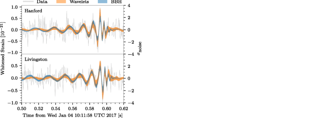
赤線がハンフォード観測所の観測データから抽出した重力波、緑線がリビングストン観測所の観測データから抽出した重力波になります
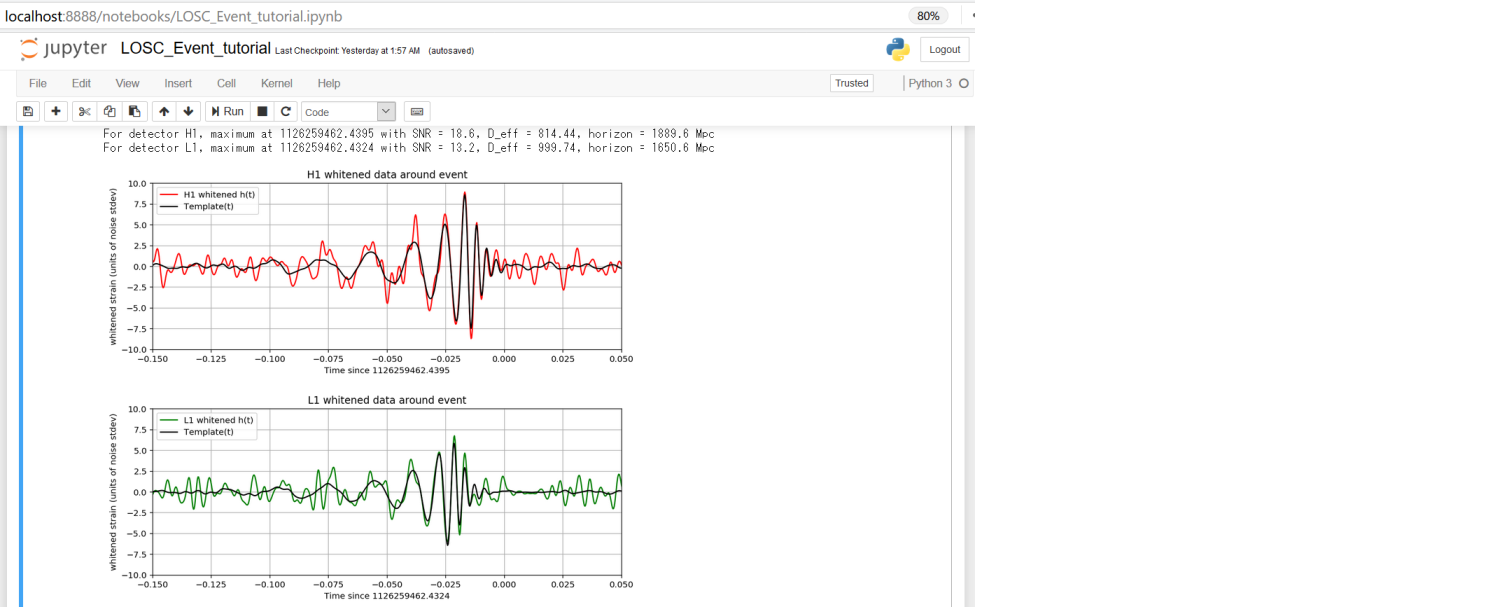
重ねた黒線は予測波形で、ほぼ予測した通りの動きになっていることが確認できました ![]()
次はあなたの手元で
このような、素晴らしいデータと解析プロセスを公開してくれたLIGOの心意気に感謝しつつ、「オープンデータが日常」となるような技術発展を遂げた、この時代に生きられたことは、本当に嬉しいことだと思います ![]()
ここまで見てきた「GW170104」と、ほぼ同じ形で、「GW150914」、「LVT151012」、「GW151226」という、あと3つの重力波データがあるので、ぜひお手元にてAnacondaをインストールして、Jupyter Notebookによる重力波の解析にチャレンジしてみてください ![]()
重力波の「その先」
最後に、重力波発見で拓かれた、近未来のSFチックな可能性をご紹介して締めくくります
①重力コントロールの可能性
「インターステラー」という映画をご存知でしょうか?

この映画の中で、ブラックホールに吸い込まれた主人公が、重力の秘密を解くために、「事象の地平線」を越えて、全ての物理量が圧縮された特異点の領域の量子データを取り、それを地球に残された娘に送り、娘が相対性理論と量子論の融合に成功し、重力コントロールの技術を得る、というシーンがあります
その技術を用いて、人類は、「スペースコロニーの建造」が可能となり、惑星移住せずとも滅亡を免れる訳です
実際には、ブラックホールに吸い込まれて無事な訳が無いためフィクションなのですが、これが「大型ブラックホールに吸い込まれつつある小型ブラックホール」であれば、ノンフィクションの世界になります
その事象を解析し、重力の謎を解明する際は、恐らく重力波がカギとなるでしょう ![]()
このコンセプトは、「重力波で見える宇宙のはじまり」という本にあるので、ご興味あれば読んでみてください

②4次元を超える次元発見の可能性
「重力」は、次元の壁を超えられる唯一の存在と言われており、私達がいる4次元(3次元空間+時間)より上の次元は、重力波から見つかる可能性あります ![]()
一般相対性理論と量子力学を融合する候補、「超弦理論」について調べてみると楽しいと思います

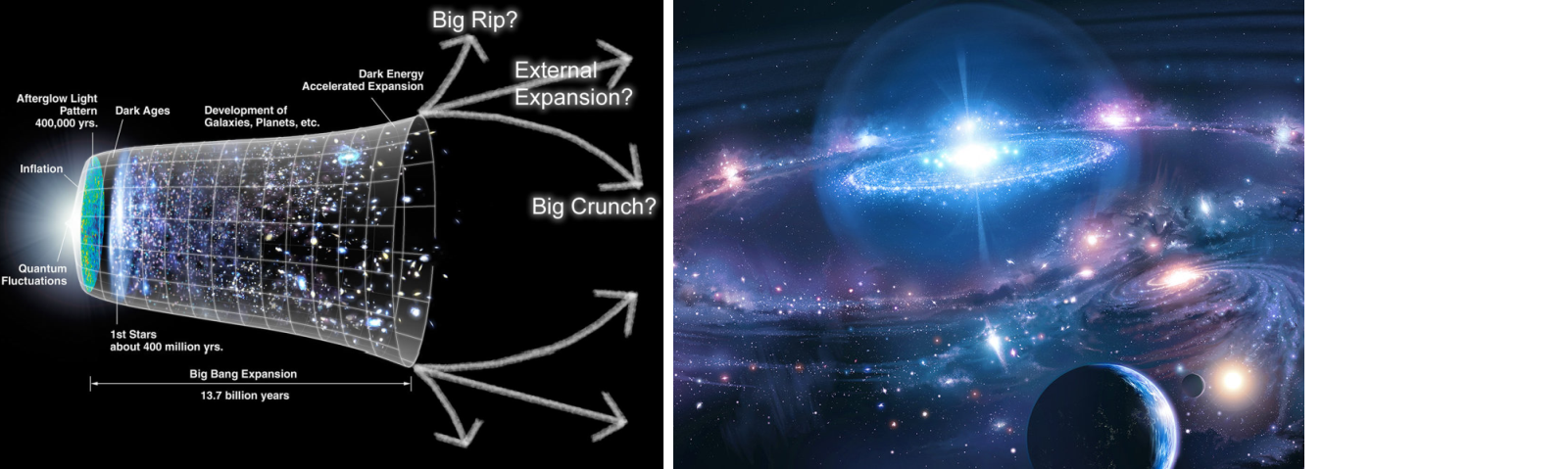
③宇宙の誕生を解明する可能性
「原子重力波」と呼ばれる、宇宙の始まりに発せられた重力波を見つけることで、宇宙の誕生を明らかにできる可能性もあります
これらの可能性が、今後、解明されていくと考えると、今から非常に楽しみで仕方ありません ![]()
p.s.
本記事に連動したLT・セッションを、福岡(天神か小倉付近)で数回、登壇します

次回登壇は、Twitterでアナウンスしますので、ご興味あればフォローください
(Elixir/ビッグデータ分析/AI・機械学習/量子コンピュータ/技術未来予測/BLAME!もツィートしてます)
最後まで、ご清聴ありがとうございます
【お知らせ】 今月12/22(金)開催の「fukuoka.ex #4」、満員御礼 
プログラミング初級者でもとっつきやすい関数型言語「Elixir」とWebフレームワーク「Phoenix」でビッグデータ分析(大量データ処理、AI・機械学習エンジンとの連携)のセッションします
「膨大なデータとアクセスの高速処理」と「高い柔軟性・開発効率」、「プログラミングの楽しさ」の全てを実現できるElixir/PhoenixのMeetUpを、隔月開催していますのでどうぞ