[論文メモ]Neural Factorization Machines #Python

読んだ論文

Xiangnan He and Tat-Seng Chua, Neural Factorization Machines for Sparse Predictive Analytics, In Proceedings of SIGIR '17, 2017
Link: https://www.comp.nus.edu.sg/~xiangnan/papers/sigir17-nfm.pdf

TL; DR

カテゴリ同士のEmbeddingをelement-wiseに掛け合わせてそれをDense層に入れたFM

この手法のやりたきこと

non-linearかつ複雑な特徴量同士のinteractionを捉える

この論文では①レコメンドのようにsparseなデータセットの場合特徴量同士のinteractionを用いることで効率的に学習できるというのが基本認識。
その上で②Factorization Machinesにおけるinteractionの捉え方はlinearでありその点が限界、という問題意識がある。
Neural Factorization Machines（以下NFM）では特徴量同士のinteractionをnon-linearかつ複雑な形でも捉えることができると主張している。

仕組み

入力$\boldsymbol{x}$と出力$\hat{y}$を考えたとき以下のように定式化される。

\hat{y}(\boldsymbol{x}) = w_0 + \sum_{i=1}^n w_i x_i + f(\boldsymbol{x})

ただし$\boldsymbol{w}$は重みで、$f(\boldsymbol{x})$は交差項である。この二項目の交差項がこの手法のキモとなっている。

Embedding Layer

この二項目の部分のイメージは以下の通り（元論文p.4より）

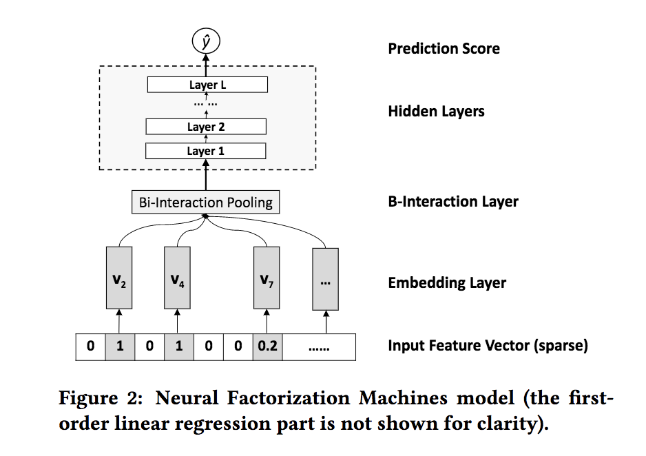
ここで何をしているのかざっくりまとめると以下の通り。

特徴量からEmbedding Layerを作成

各特徴量のEmbedding Vectorをelement-wiseに掛け合わせる

element-wiseに掛け合わせたEmbedding VectorをDense層に入れる（複数層を重ねても良い）

すごく雑に言うとFMの交差項をNNに入れ込んだだけ。
上の図に合わせて式で表すと以下のようになる。

\begin{align}
\hat{y} &= \boldsymbol{h}^T \boldsymbol{z}_L \\
\boldsymbol{z}_L &= \sigma_L \bigl(\boldsymbol{W}_L \boldsymbol{z}_{L-1} + \boldsymbol{b}_L \bigr) \\
... \\\
\boldsymbol{z}_2 &= \sigma_2 \bigl(\boldsymbol{W}_2 \boldsymbol{z}_1 + \boldsymbol{b}_2 \bigr) \\
\boldsymbol{z}_1 &= \sigma_1 \bigl(\boldsymbol{W}_1 f_{BI}(\boldsymbol{V}_x ) + \boldsymbol{b}_1 \bigr) \\
f_{BI}(\boldsymbol{V}_x ) &= \sum_{i=1}^n \sum_{j=i+1}^n x_i v_i \odot x_j v_j
\end{align}

一番最後がEmbedding Vector化した特徴量をelement-wiseに掛け合わせたもので、これがsecond-order interactionだとのこと（この点もう少しきちんと言葉を詰めたい）。
なお通常のFMと同じく実際の計算のときはコストを抑えるため最後の式を以下のように変形する。

f_{BI}(\boldsymbol{V}_x ) = \frac{1}{2} \Bigl[ \bigl(\sum_{i=1}^n x_i v_i \bigr)^2 - \sum_{i=1}^n (x_i v_i)^2 \Bigr]

変形の過程はFMのときと全く同じ。

NFMとFMの関係

FM is a shallow and linear model,which can be seen as a special case of NFM with no hidden layer.とあるようにNFMはFMの一般形であるとこの論文は主張している。
実際L=0のケース（element-wiseに掛け合わせたあとNNに投入しない）を考えると以下のように式が展開される。

\begin{align}
\hat{y}(\boldsymbol{x}) &= w_0 + \sum_{i=1}^n w_i x_i + \boldsymbol{h}^T f_{BI}(\boldsymbol{V}_x ) \\
&= w_0 + \sum_{i=1}^n w_i x_i + \boldsymbol{h}^T \sum_{i=1}^n \sum_{j=i+1}^n x_i v_i \odot x_j v_j \\
&= w_0 + \sum_{i=1}^n w_i x_i + \sum_{i=1}^n \sum_{j=i+1}^n \sum_{f=1}^d h_f v_{i,f} v_{j,f} \odot x_i x_j \\
\end{align}

ここで$\boldsymbol{h}^T$を(1,1,...,1)という定数のベクトルと置くことでNFMをFMに戻すことができる。

実装

著者本人による実装がこちらのGitHubリポジトリにアップされている。
元の実装は生tf使っておりかつRegression問題に対するものであったため、今回はEstimatorを用いた分類問題のものに少しだけ変形。
使用したnotebookはこちら。

今回も用いているデータセットはMovieLens20M。
Wide and Deep¹のときと変更すべき点はカラムのデータ型定義のところとmodel_fnのみ。
まずはデータ型定義のところを確認

# Embeddingのdimensionを設定
user_embedding_dim = 256
item_embedding_dim = 256

# カラム情報取得
categorical_hash_user_raw = \
tf.feature_column.categorical_column_with_hash_bucket('user_id', CATEGORICAL_FEATURE_NAMES_WITH_BUCKET_SIZE['user_id'])
categorical_hash_item_raw = \
    tf.feature_column.categorical_column_with_hash_bucket('item_id', CATEGORICAL_FEATURE_NAMES_WITH_BUCKET_SIZE['item_id'])

# 前半のlinearパート　→　結局使ってない
categorical_hash_user = tf.feature_column.indicator_column(categorical_hash_user_raw)    
categorical_hash_item = tf.feature_column.indicator_column(categorical_hash_item_raw)
categorical_feature_linear = [categorical_hash_user, categorical_hash_item]

# 後半のEmbeddingパートを作成
categorical_feature_user_emb = tf.feature_column.embedding_column(
    categorical_column=categorical_hash_user_raw, dimension=user_embedding_dim)
categorical_feature_item_emb = tf.feature_column.embedding_column(
    categorical_column=categorical_hash_item_raw, dimension=item_embedding_dim)
categorical_feature_emb = [categorical_feature_user_emb, categorical_feature_item_emb]

このあたりはいつものEstimatorのときとあまり変わらない。
今回Custom Estimatorを作成するにあたり以下のような辞書を作成。

params = {
    'categorical_feature_linear': categorical_feature_linear,
    'categorical_feature_emb': categorical_feature_emb,
    'hidden_units': [128, 64, 32],
    'dropout_prob': 0.3,
    'n_classes': 2
}

いよいよNFMのmodel_fn。
まずは特徴量の入力から交差項の作成部分まで

# paramsを元に使用する特徴量を選択
# featuresはinput_fnより出力されるtensor
input_features_linear = tf.feature_column.input_layer(features, params['categorical_feature_linear'])

input_features_dnn = tf.feature_column.input_layer(features, params['categorical_feature_emb'])

# sumの二乗    
feature_sq_sum = tf.square(tf.reduce_sum(input_features_dnn, axis=1, keepdims=True))
# 二乗のsum
feature_sum_sq = tf.reduce_sum(tf.square(input_features_dnn), axis=1, keepdims=True)
# 交差項
cross_term = 0.5 * tf.subtract(feature_sq_sum, feature_sum_sq)

ここで作成した交差項cross_termをNNに入れ込んでいく

for hidden_unit in params['hidden_units']:
    layer = tf.layers.dense(cross_term, units=hidden_unit, activation=tf.nn.relu)
layer = tf.nn.dropout(layer, rate=params['dropout_prob'])
logits = tf.layers.dense(layer, params['n_classes'], activation=None)

あとは評価の部分なので詳細な説明は割愛。
このmodel_fnの全体像を示すと以下の通りになる。

def NeuralFM_fn(features, labels, mode, params):
    input_features_linear = tf.feature_column.input_layer(features, params['categorical_feature_linear'])
    input_features_dnn = tf.feature_column.input_layer(features, params['categorical_feature_emb'])

    feature_sq_sum = tf.square(tf.reduce_sum(input_features_dnn, axis=1, keepdims=True))
    feature_sum_sq = tf.reduce_sum(tf.square(input_features_dnn), axis=1, keepdims=True)
    cross_term = 0.5 * tf.subtract(feature_sq_sum, feature_sum_sq)

    for hidden_unit in params['hidden_units']:
        layer = tf.layers.dense(cross_term, units=hidden_unit, activation=tf.nn.relu)
    layer = tf.nn.dropout(layer, rate=params['dropout_prob'])
    logits = tf.layers.dense(layer, params['n_classes'], activation=None)

    predicted_classes = tf.argmax(logits, 1)
    if mode == tf.estimator.ModeKeys.PREDICT:
        predictions = {
            'class_ids': predicted_classes[:, tf.newaxis],
            'probabilities': tf.nn.softmax(logits),
            'logits': logits,
        }
        return tf.estimator.EstimatorSpec(mode, predictions=predictions)

    loss = tf.losses.sparse_softmax_cross_entropy(labels=labels, logits=logits)

    accuracy = tf.metrics.accuracy(labels=labels,
                               predictions=predicted_classes,
                               name='acc_op')

    metrics = {'accuracy': accuracy}
    tf.summary.scalar('accuracy', accuracy[1])

    if mode == tf.estimator.ModeKeys.EVAL:
        return tf.estimator.EstimatorSpec(
            mode, loss=loss, eval_metric_ops=metrics)

    optimizer = tf.train.AdamOptimizer()
    train_op = optimizer.minimize(loss, global_step=tf.train.get_global_step())
    return tf.estimator.EstimatorSpec(mode, loss=loss, train_op=train_op)

一応著者本人のを見て作成したものの、一項目（Linearのパート）の記述がどこにも見当たらず二項目のFM部分しかなかった。
うーんこれでよいのかちょっと自信ない。

評価

ひとまず今回は以下のような四通りのパターンで評価

user_hash_bucket_size, item_hash_bucket_size: {1000, 10000}
user_embedding_dim, item_embedding_dim: {128, 256}

hidden_unitsはWide and Deepのときと同じ（[128, 64, 32]）だがDropoutは最後のDense（出力の一個前）にのみ設けている。Dropout rateは同じく0.3。
結果は以下の通り。

	bucket_size=10000	bucket_size=20000
emb_dim=128	0.7054	0.7191
emb_dim=256	0.7057	0.7246

うーんどうも他の特徴量入れてないとFMよりよくならない。なぜだ...。
時間見つけてもっとパラメータをいじってみよう。

謎が深まるばかりであまり閉まらないがひとまず以上。お粗末！

手前味噌だがこちらのnotebookからWide and Deepのコードを確認できる。。 ↩